Learn with Us
It's exciting to start your own journey to solve bioinformatics problems. Learn these skills and enjoy! Please follow these protocols
Study Protocols
NCBI and BLAST
AIMS:
To search for homologs of the cathepsin L protein sequence using NCBI and BLAST.
OBJECTIVES:
- To understand the concept of homology
- To get acquainted with a simple biological sequence file formats (FASTA and GenPept)
- To retrieve a human cathepsin L protein sequence in FASTA format
- To retrieve 8 homologs of human cathepsin L using NCBI BLAST
EXPECTED OUTCOMES:
- To get a general understanding of NCBI web resource
- To be able to query a biological sequence database using BLASTP
- To understand the BLAST report
PRIOR PROTOCOL(S) REQUIRED FOR THIS PROTOCOL:
N/A
SUGGESTED NEXT STEP(S):
Multiple sequence alignment
Introduction
As part of a study on the role of cathepsin L on protein turnover in humans, we are to choose a suitable sequence from the NCBI website. We also have to determine what the function of the protein is and report other features associated with the protein. Additionally, we will retrieve similar (homologous) copies of the protein sequence in other organisms, before proceeding to further analysis.
Your first task is to retrieve information from the National Center for Biotechnology Information(NCBI) website, which can be found at the following url http://www.ncbi.nlm.nih.gov/. NCBI (hosted at the National Library of Medicine) stores different types of biological information in various databases and has various tools for sequence retrieval and visualization. We will begin our investigation by selecting the “protein” database in the search bar using the term “cathepsin L” AND “human”[orgn]. This type of search uses both a filter [orgn] and a boolean “AND” and this crafted search will only return entries where the term “cathepsin L” is linked to the term “human” defined as an organism. As we intend to do structural analyses later on, we will therefore filter the returned results by clicking the PDB database option on the left of the page.
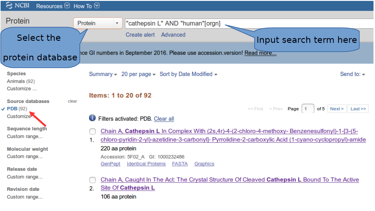
Note that each of the returned results is linked to the human as an organism and that these results would be less specific had the organism filter “[orgn]” not been used.
Examining the results
Let us examine the first result by clicking on it's link.
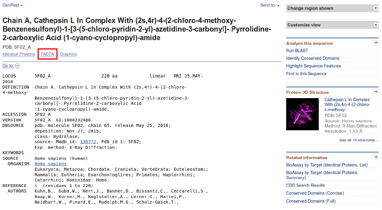
The NCBI record (from the Genbank database of NCBI) returned is in GenPept format. This format associates various annotations as headers to the protein sequence it contains, further below. You can verify that the source organism denoted by the keyword “ORGANISM” is indeed a human (Homo sapiens). Notice the associated PDB structure on the right of the web page.
It is important to note that not all sequences from NCBI are “curated”, i.e. verified by expert knowledge and not just labeled by automatic computer predictions. An example of a curated sequence database is RefSeq (reference sequence database). In our case our sequence is linked to a crystal structure and a puplication, we therefore know that the sequence is not a possible erroneous result from a computational inference from a stretch of nucleic acid.
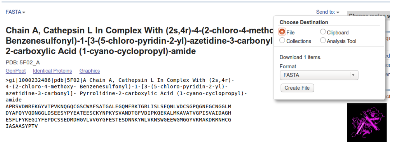
Next, click on the FASTA (in red) link on the GenPept report. This will return the sequence in FASTA format - the first line starts with a “>” describing the sequence, followed by the sequence on the following lines. Save the file to your computer (preferably on the desktop) by clicking on “send to”, followed by “File → FASTA → create file”. Important: Save the file to your desktop. It will be used in a later section.
You can also copy only the sequence or copy the entire FASTA record, including the “>” symbol, for what we will do next.
Basic Local Alignment Search Tool(BLAST)
BLAST, which stands for “Basic Local Alignment Search Tool” finds database matches (potential homologs) against a given query sequence.
The NCBI BLAST interface changes periodically, but the main things to remember are the main variants of the BLAST search tools, namely BLASTN, BLASTP, BLASTX, TBLASTN and TBLASTX. BLASTN searches a nucleotide database, given a nucleotide query. BLASTP searches a protein database, given a protein query. BLASTX searches a protein database given a nucleotide (translated) query. TBLASTN searches a translated nucleotide database using a protein query. For TBLASTX both query and database sequences are translated nucleotides. For our purposes, we will simply use BLASTP. In all cases, hits (matches or subjects) are returned as a list on the basis on “similarity” metrics of local sequence alignments. Similarity, in this case should not be confused with the BLAST calculation for similarity.
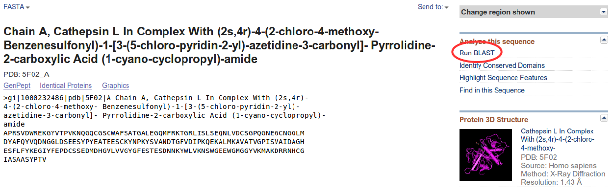
Click on any of the links leading to the BLAST tool. Set the database to PDB, so that the hits obtained have matching structural information. PDB (Protein Data Bank) will be covered in a later section. The BLAST interface also works with accession numbers (unique identifiers) as input, but you can try replacing this identifier with your sequence (see below).
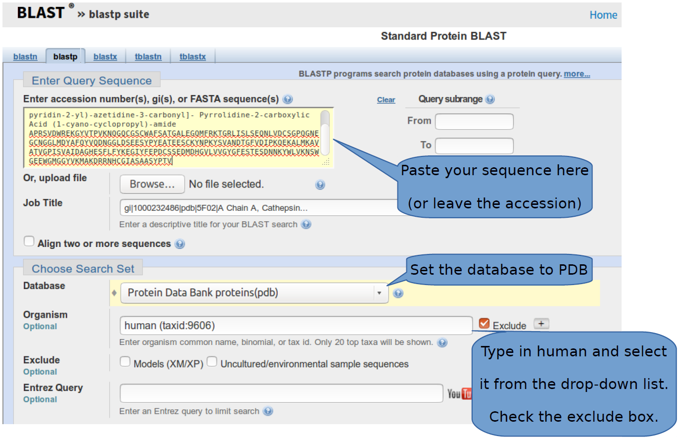
Exclude human sequences as shown in the above figure. Scroll down and check the “Show results in a new window”. Click “BLAST” on the lower left corner. These parameter selections exclude any human sequence and focus the search only on those linked to structures in the PDB database. A new tab will be opened and the page will refresh a few times until the results are ready to be displayed.
Search Results
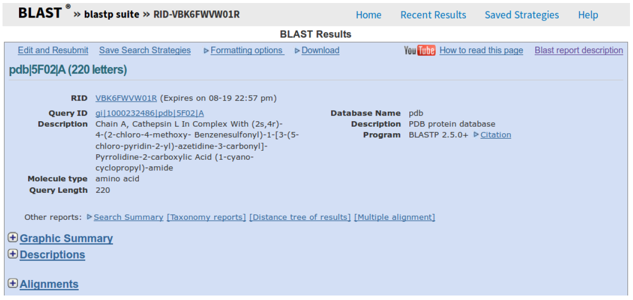
The BLAST report page (figure below) is very comprehensive and gives details of the hits as a graphical summary. Corresponding hit statistics and the actual (local) alignments to the hit database sequences are also included.
Help pages and videos are available for further documentation.
BLAST, which stands for “Basic Local Alignment Search Tool” finds database matches (potential homologs) against a given query sequence.
The graphic summary (next figure) gives you a quick overview of how well each matched database sequence is aligning to the given query sequence. The whole query is just under the color key, and the color of the hits (below) hints about the quality (score) of the alignment.
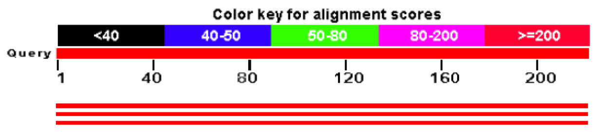
Clicking on any of the hits sends you to the alignment, if you want to examine the actual differences and/ or identities between your query and hit.
Two sequences are said to be homologous if they come from the same “ancestor”. The ancestor in this case is the common gene or biological sequence from which the currently observed sequences are expected to have descended, via the process of evolution. In the search for homologs, we want hits that have the lowest E-value (<1e-4), the highest coverage and highest percentage identity. The BLAST similarity metric basically gives the percentage of residues that share similar physicochemical properties. A scoring matrix is used for matter. Sequence identity simply calculates the percentage of identical residues between the query and the hit sequence. If you are unfamiliar to the notation, 1e-4 = 0.0001.
Q1. Scroll down to the “Descriptions” section and click on the first hit. This brings you to the alignment section. Click on the “Sequence ID” link – this opens a new web page, which shows linked information to the hit in GenPept format. Search for the keyword ORGANISM and report the organism name.
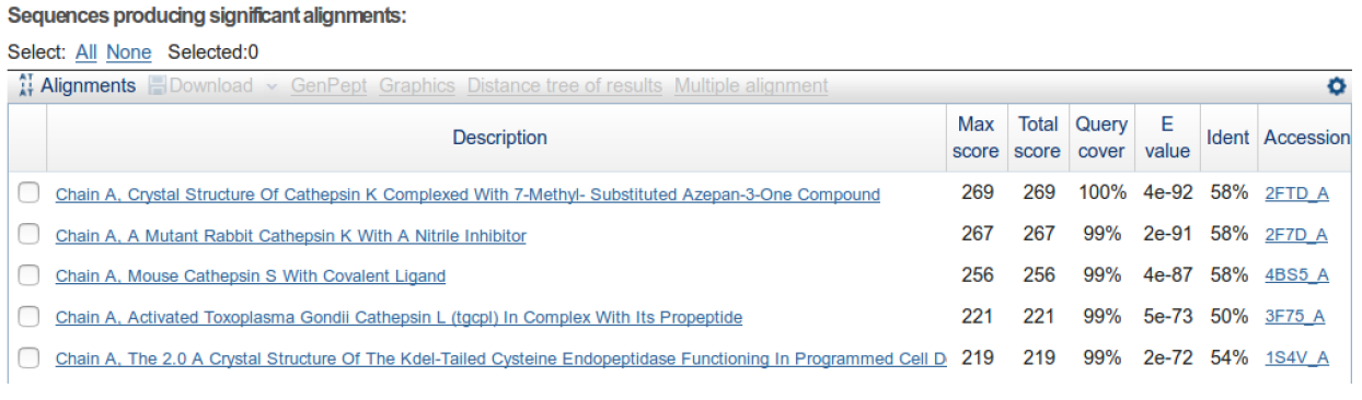
Q2. Go to back to the the graphic summary and click on the first pink bar amongst the hits. Which organism does it belong to?
Q3. A domain is an independent functional unit within a protein and is conserved if it is found relatively unchanged across several different organisms. According to the BLAST report, which conserved domain superfamily was detected? (Scroll up on the BLAST report page)
Let us now quickly see which organisms have potential homologs of the protein. Scroll to the top of the BLAST report page and click “Distance tree of results”.
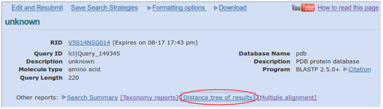
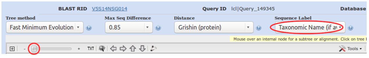
A phylogenetic tree is generated on a new web page, with default parameters. The tree is good only for visualizing the hits at first glance, but very careful analysis of the alignments is needed for any strong biological inference. Click the “Sequence Label” tab, choose “Taxonomic Name (if available)”. Then drag the zoom slider to the right, until you can see the taxon names on the tree.
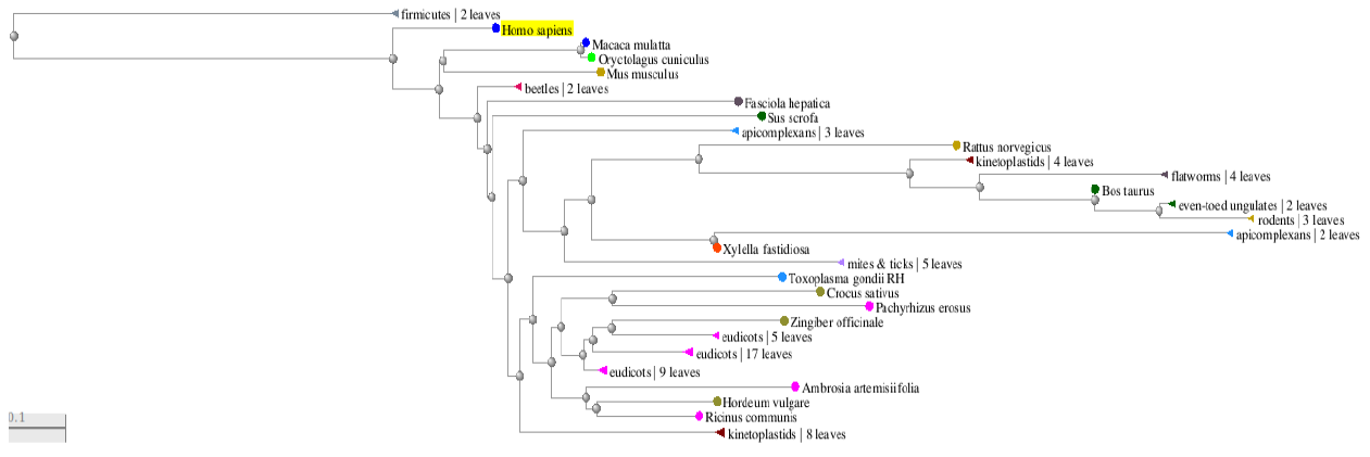
The tree is composed of nodes (termed “taxa”, where lines end and also where they intersect) and branches (the lines connecting the taxa). Click and drag the image to navigate along the tree branches.
Hover your mouse over the “apicomplexans” node (triangle) and click “expand”. Indeed, it is quite interesting to find that these malarial parasites share similar proteins to us! Also notice the presence of the toxoplasmosis-causing pathogen, against which there is no effective human vaccine to date. This can indeed set the stage for interesting bioinformatics research. At time of writing, the tree obtained was as shown in the figure below. It will change with time, as new sequences are added to the NCBI PDB repository.
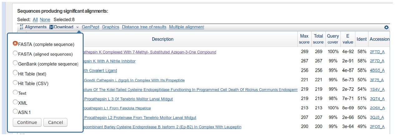
Now, let's choose members of the apicomplexans, kinetoplastids and the Toxoplasma hit. Switch back to the “Descriptions” section from BLAST report page and select each box corresponding to these 8 accessions: 1YVB_A, 3PNR_A, 3BPM_A, 4XUI_A, 4W5C_A, 3HD3_A, 2P7U_A, 3F75_A.
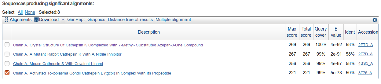
Then click Download → FASTA (complete sequence) → Continue:
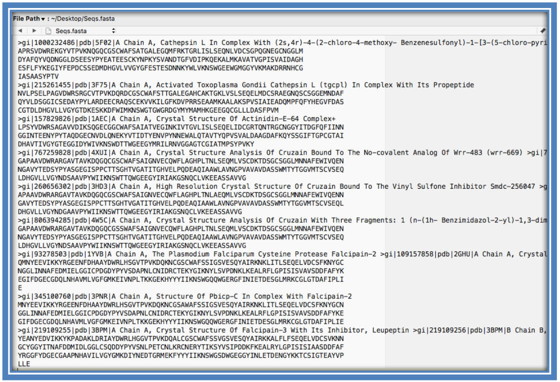
Save the file to your Desktop. At the end of this section, you should have a file with your initial human cathepsin L sequence and another file containing the 8 non-human homologs.
Multiple sequence alignment (MSA)
AIMS:
To analyze homolog protein sequences at sequence level to identify the conserved regions as well as closely related ones.
OBJECTIVES:
- To analyze various MSA programs to identify the most accurate program for your sequence alignment
- To calculate pairwise sequence identities
- To identify conserved and non-conserved regions within the homolog sequences
EXPECTED OUTCOMES:
- To be able to align homolog sequences in protein format
- Understand various alignment algorithms
PRIOR PROTOCOL(S) REQUIRED FOR THIS PROTOCOL:
Retrieval of homolog sequences and 3D structures (See, NCBI, BLAST, HHPRED sections)
SUGGESTED NEXT STEP(S):
Mapping the conserved regions to 3D protein structures (See PDB, visualization of protein structures and Homology modeling sections)
Background
An alignment can be carried out on either protein or nucleic acid sequences (aligning protein sequences with protein sequences and nucleic acid sequences with nucleic acid sequences). A pairwise sequence alignment (alignment of 2 sequences) is often not as informative as a multiple sequence alignment, MSA (alignment of several sequences). Areas of similarity often indicate conservation between the sequences, however, this can be observed better in a MSA than a pairwise sequence alignment. This similarity can be linked to evolution, structure or function.
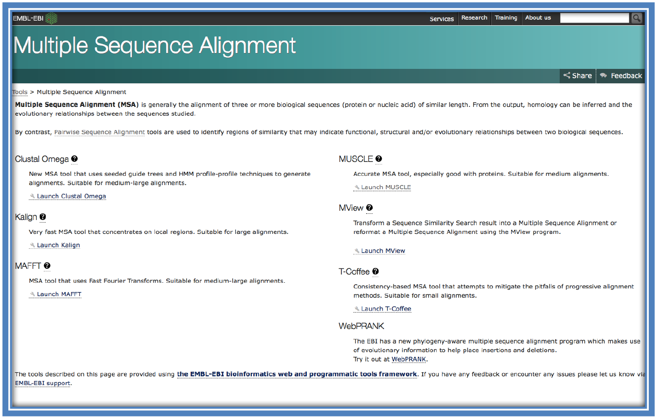
There are two main forms of multiple sequence alignment algorithms; global and local alignments. Global alignment algorithms compare whole sequences to each other from end to end (e.g. LALIGN, Kalign). These are most useful when sequences are the same length. Local alignment algorithms align sections of the sections which match more closely. Local alignments are usually better suited when using sequences of different length and when looking for regions of conservation within a given sequence (e.g. LALIGN). Some of the most popular/trusted programs used to perform multiple sequence alignments can be found on the EBI website (http://www.ebi.ac.uk/Tools/msa/).
Sequences are aligned with the chosen algorithm by the various programs available (e.g. MAFFT, MUSCLE, PROMALS3D, 3DCOFFEE). The outputs of each program are generally presented in a similar manner with the aligned sequences each shown on a separate line. Residues (or nucleotides in the case of a nucleic acid sequence alignment) are stacked in columns and match up with the position of the residue below in the same column. In the occurrence of a residue not matching a dash (“-“) is generally inserted creating a “gap”. This ensures future matching residues line up in the same columns.
Since structure is often more conserved it is useful to use known structures to construct multiple sequence alignments (e.g. PROMALS3D and 3D-COFFEE). This type of alignment aligns the sequences to the structure provided and takes into account the constraints imposed on the structure during an alignment (e.g. often gaps are not inserted in secondary structures such as alpha helices and beta sheets)/ To use this method refer to the section on the PDB and protein structure retrieval. Most of these programs do not require you to have downloaded the protein structure but you would then need to know its PDB ID (unique identifier of the structure within the Protein Data Bank of available structures).
There are many programs available to visualize MSA’s e.g. Jalview and UGENE. These programs make it easier to distinguish the conserved regions as well as the areas of distinction by using specific coloring tools (e.g. ClustalX coloring – shows each residue colored according to type – columns of matching color can then be quickly identified as conserved).
Sequences to align
STEP 1:
Follow the steps from the BLAST protocol to retrieve the sequences that you would like to align. These sequences should be in FASTA format in one file. It is recommended to use a text editor such as Notepad or Wordpad since programs such as Word or Office might change the formatting.
STEP 2:
There are many different MSA programs available. For this tutorial we will only consider those that use webservers (i.e. can be completed online without any program installations or downloads). Many of the programs are available through the EBI-Suite (http://www.ebi.ac.uk/Tools/msa/).
Select a MSA program to use. Consider things such as;
- Do you have a 3D structure which could be used with the MSA? (In which case you could use PROMALS3D which uses the protein structure during the alignment process)(http://prodata.swmed.edu/promals3d/promals3d.php)
- Are the sequences the same length or different? (This would influence whether to perform a global or a local alignment)
- Are the sequences closely or more distantly related?
It is generally recommended to use more than one program for the MSA step and then assess the final alignments to determine which was the best MSA of the data. For this it is often helpful if you have a bit of knowledge on your sequence/ protein (e.g. if you know there is a conserved region you can ensure this region was not altered in the alignment).
MUSCLE as an example
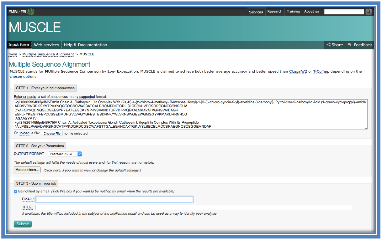
STEP 3:
Once you have selected the program(s) you will be using to carry out the MSA insert your sequences into the allotted box (in FASTA format) or upload the file of your sequences (in FASTA format). Select the format you would like the results outputted in (FASTA format is recommend – this would mainly depend on the visualization program you would be using at a later stage). Use the default parameters. Features should only be changed if you know specifically what they are for. You are encouraged to add your email address so the results may be sent to you on completion. This is helpful if you lose the page or loose internet etc. It can also be useful if you need to come back and look at the data at a later stage. Do take note on the various webservers and how long they will store your results for to ensure you save a copy before it is removed. Submit the job.
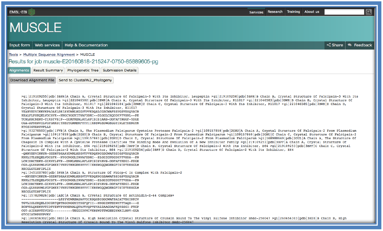
STEP 4:
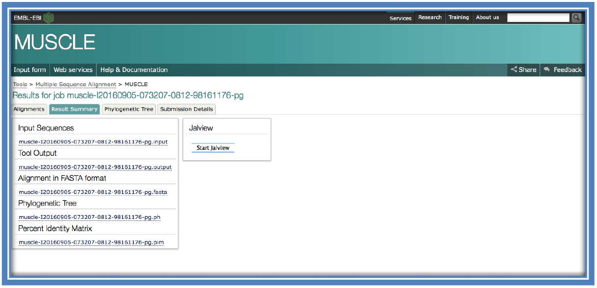
Once the MSA has finished running and your results are returned you should get something similar to the image below. Save the alignment (in FASTA format).
STEP 5:
When looking at the returned page there will be a tab on the page entitled “Result Summary”.
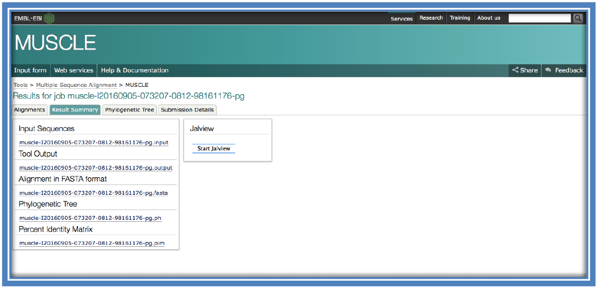
This will show many different options that can be selected from there other than just the alignment (which can be viewed in the Alignments tab or here under “Alignment in FASTA format”) such as “Phylogenetic Tree” and “Percentage Identity Matrix” (See steps 10 & 11).
Viewing the alignment
STEP 6:
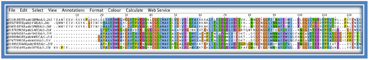
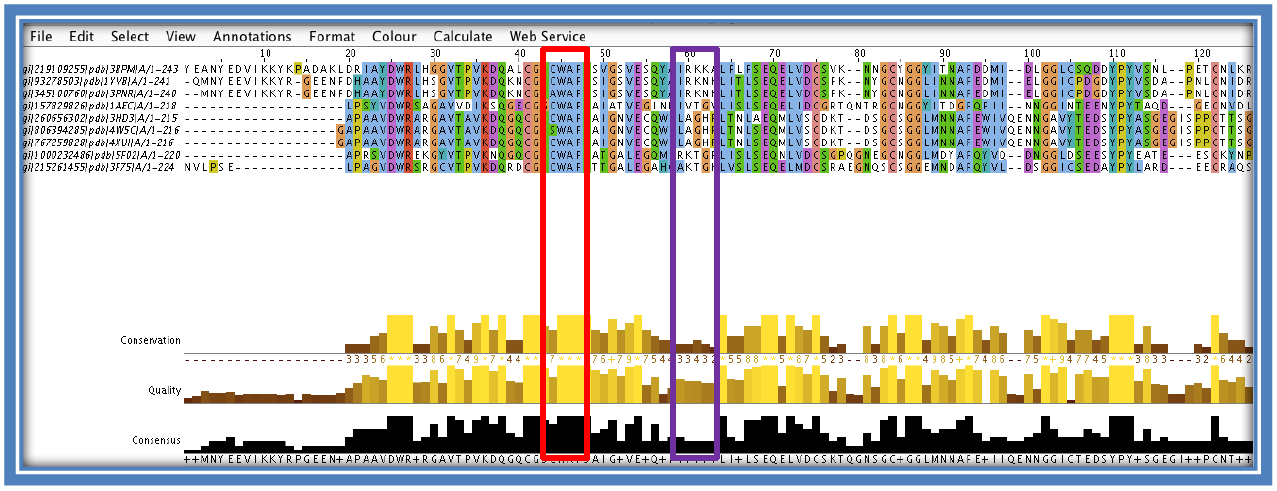
The alignment can be viewed by clicking on “Start Jalview” on the Result Summary tab (if Java is not loaded you can also use the alignment viewer part of the Bioinformatics Toolkit developed by the Max Plank Institute: https://toolkit.tuebingen.mpg.de/alnviz see step 12). This will load a pop-up applet. Here you will be able to visually see the areas of conservation. The coloring can be changed to see different features such as; identical amino acids in columns, coloring according to percentage identity, hydrophobicity etc.
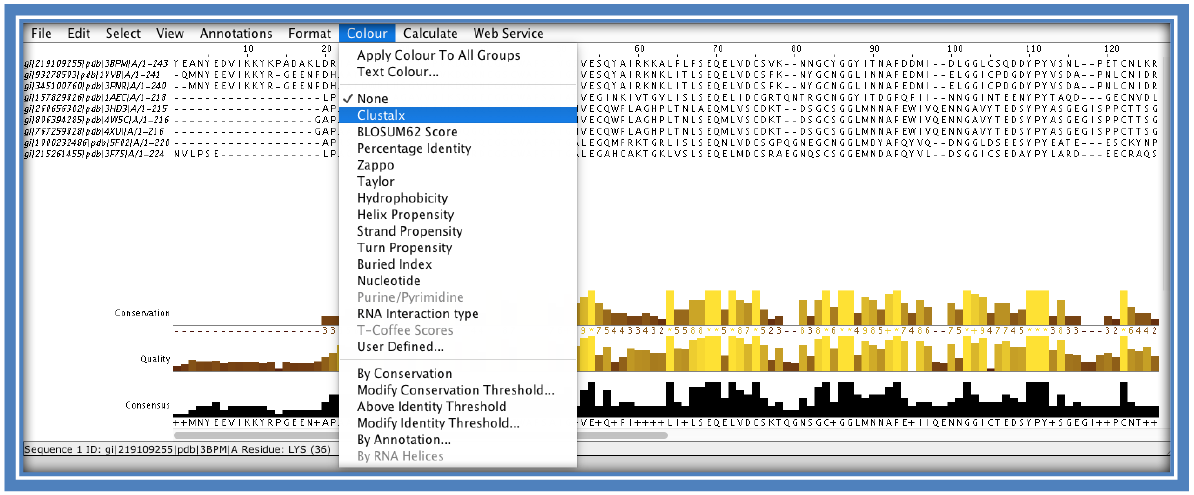
STEP 7:
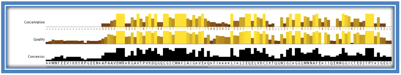
The histograms under the alignment also give a visual representation of the MSA in the form of 3 histograms; conservation, quality and consensus. These are automatically calculated by Jalview on loading the MSA.
- - The “conservation” histogram:
- This calculation is a quantitative measure of the number of conserved physicochemical properties within that column (e.g. amount of acidic/hydrophobic etc and the more residues within that column with the same physicochemical property the more conserved over the column and the larger the histogram level).
- - The “quality” histogram:
- Is a quantitative alignment annotation showing the likelihood of a mutation occurring in that particular column. A high column in this histogram would indicate there are no mutations in that column/ at that position or that any which do occur are considered to be favorable.
- - The “consensus” histogram:
- Shows the percentage of the modal (most occurring) residue in that column. Gaps are included in this calculation. A “+” symbol is used to indicate that there is more than one modal residue at that position (at least 2 residues occur the same amount of times – more than the others).
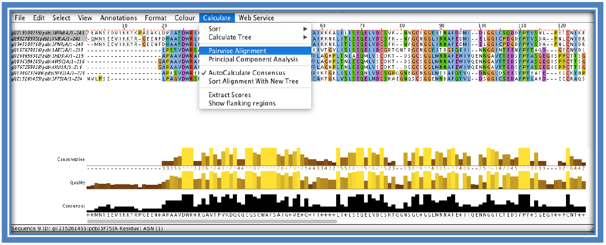
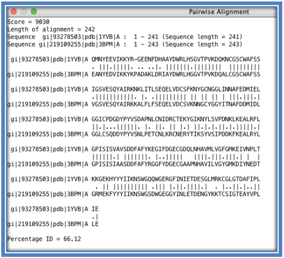
STEP 8:
Calculate the sequence identity of sequences. **Sequence identity is calculated as a percentage as the amount of residues that are identical between the two sequences being compared on a position/column basis. This is generally done on a pairwise basis comparing one sequence to another. Jalview does allow the user to select all the sequences and perform a pairwise sequence identity calculation. The output file will show a pairwise alignment of each sequence to each other possible sequence in the set as well as the final sequence identity percentage.
STEP 9:
Examine the results. Columns with matching colors and corresponding high histograms will show conservation at that position. If looking for variations between the sequence look for areas where the conservation is low or gaps had to be inserted. The red box below shows higher conservation between the sequences with the purple box showing a region of more variation.
STEP 10:
Back to the “Result Summary” page.
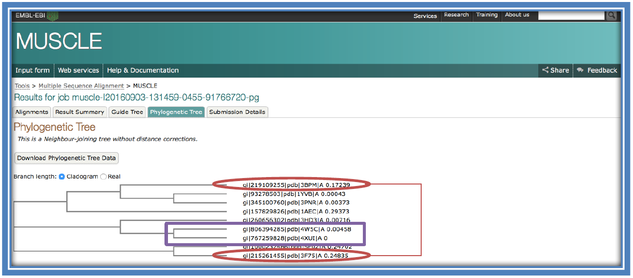
Here there is a result generated for the “Phylogenetic Tree”. That link will take you to a page as below. This shows how closely related the different sequences are to each other. Closely connected sequences are more closely related (purple box) while sequences on different branches are less related (red ovals).
STEP 11:
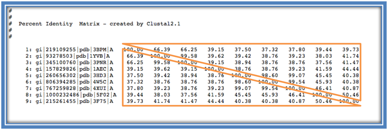
Back to the “Result Summary” page as before. Here there is a result generated for the “Percentage Identity Matrix”.
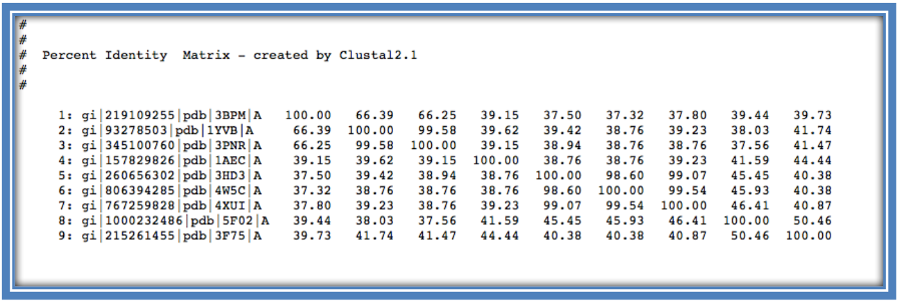
This shows the percentage identity of each of the sequences to each other sequence in the alignment (similar to Step 8 using Jalveiw). Across the diagonal of the matrix each sequence is compared in a pairwise alignment with itself and therefore generates a percentage identity of 100%. The matrix is therefore a mirror image of itself across the diagonal (as seen below in the 2 identical orange triangles).
STEP 12:
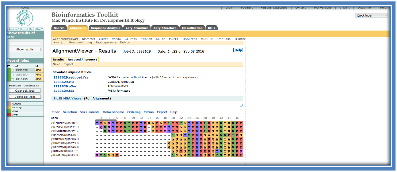
An alternative alignment viewer such as the one part of the Bioinformatics Toolkit developed by the Max Plank Institute (https://toolkit.tuebingen.mpg.de/alnviz) can also be used.
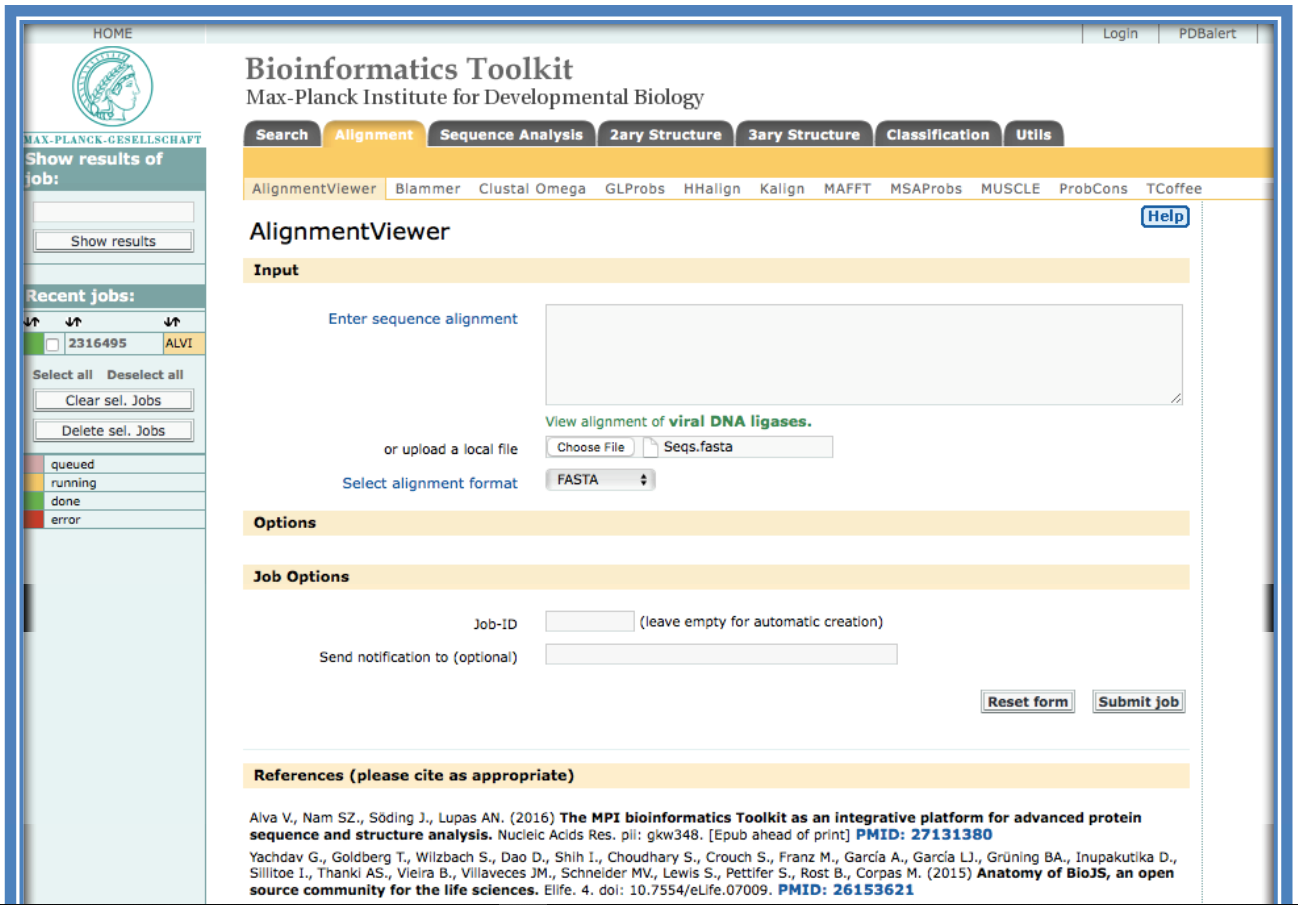
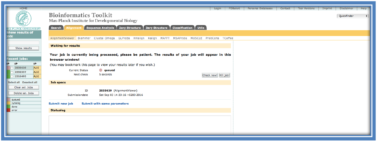
Enter the alignment generated and saved in Step 4 above. This can either be done by pasting it into the box “Enter sequence alignment” or uploading the saved file under “Choose File”. A Job-ID can be selected and an email address entered to receive the results on completion. Select “Submit job”. A loading/ running screen will be loaded while the alignment is being read.
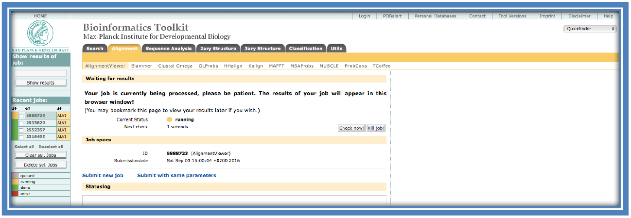
On completion the following screen will load with the alignment in the viewer.
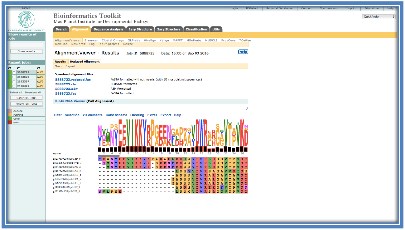
There are many options available in this alignment viewer such as; changing the color of the alignment (“Color scheme”), viewing the consensus histograms and see the sequence logo (“Vis.elements”). The consensus histograms show the consensus among the sequences at that location of the alignment. The sequence logo shows what is the most common residue at that particular position. In some cases there is more than one possible residue at a position in which cases they are shown in scale of the relation to how often they occur at that position with the most frequent occurring the largest and the least occurring the smallest. E.g. at position 26 there is only a large “W” showing this residue is conserved through all the sequences, while at position 33 there is a large “T” and a small “V” showing the there is a Threonine in 8 of the 9 sequences with one sequence having a Valine instead at that position.
Protein Data Bank (PDB)
AIMS:
Understand how to use the Protein Data Bank as an online resource.
OBJECTIVES:
- To understand the PDB summary page
- To assess the quality of structures in the PDB
- Download PDB structures
EXPECTED OUTCOMES:
- To be able to find and download structures from the PDB
- To be able to assess the quality of structures found in the PDB
PRIOR PROTOCOL(S) REQUIRED FOR THIS PROTOCOL:
None required, but PDB IDs for protein structures can be obtained in HHpred and BLAST sections
SUGGESTED NEXT STEP(S):
Use structures in homology modeling
Visualize protein structures and map motifs to structures
Further analyze protein-ligand interactions
Using the Protein Data Bank
The Protein Data Bank (PDB) is an online database of protein and nucleic acid structures that have been solved experimentally. This protocol represents a set of instructions to allow you to use the PDB website to find and download PDB structures, as well as get an understanding of the information displayed on the pages of the PDB.
There are officially three different PDB websites: the RSCB PDB (http://www.rcsb.org/pdb/), the PDB in Europe (PDBe; http://www.ebi.ac.uk/pdbe) and the PDB Japan (PDBj; http://pdbj.org/). All of these fall under the Worldwide PDB (wwPDB; http://www.wwpdb.org/) and contain the same PDB entries. Which one you use is a matter of preference, especially as far as simply finding and retrieving a structure is concerned. For the purposes of this protocol, we shall be using the RSCB PDB.
PDB ID
Before getting started, it is important to be familiar with a PDB ID. This is an identifier, consisting of four alphanumeric characters, that is unique to each PDB structure. For example, we will be looking at PDB entry 5F02, which is a structure of Cathepsin L. Related structures that are solved as part of the same experimental work will have similar PDB IDs. Note, there can be many different PDB entries for a given protein – i.e. there are many different PDB entries for Cathepsin L.
Go to the PDB website
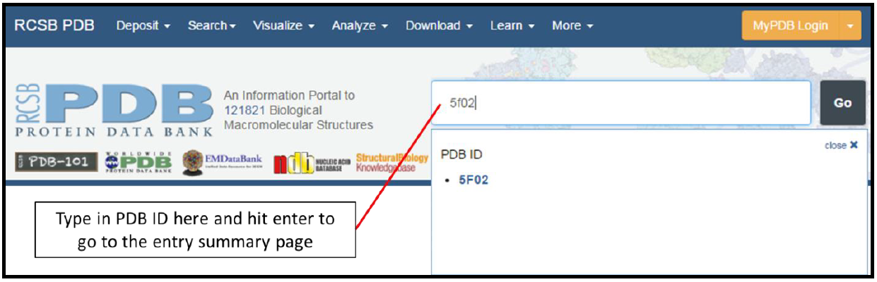
The first step of using the PDB is to go to the website, http://www.rcsb.org/pdb/. The information displayed on the home page changes frequently, but the screen clipping shown below should appear at the top of the page. Assuming you have the PDB ID of the entry you want to look at, you can use this portion of the page to search for and go to the summary page of that entry. If you do not have a PDB ID to work with, please see protocol for HHpred or BLAST.
In our example, we enter the PDB ID of Cathepsin L (5F02) into the search box and press the Enter key. This takes us to the summary page for this entry.
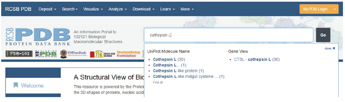
Additional search functionality
The search bar can be used to find PDB files using more than just the PDB ID. You can search based on authors, macromolecule (protein or nucleic acid) names, sequences or ligands solved. Below are two examples of this. First, by searching the name of the protein (in our case, Cathepsin), the site gives suggestions of proteins in the PDB that match this description. Shown in brackets is the number of structures that match each of these options.

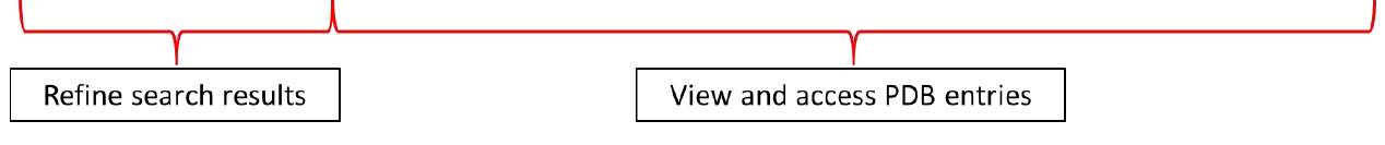
You can also search based on the sequence of the protein by pasting this into the search bar and clicking on the ‘Go’ button. This will take you to the search results page, which shows PDB entries that have sequences that are the same or similar to the sequence entered. The left hand side of the page can be used to further refine your search.

Overview
The PDB summary page
If you scroll down the summary page you will notice that a lot of information is housed here. This is summarized in the screen shot below. Essentially this contains basic information about the PDB entry, as well as literature concerning this entry, information about macromolecular entities, small molecule entities and experimental validation. Each of these sections will be explained as we go along.

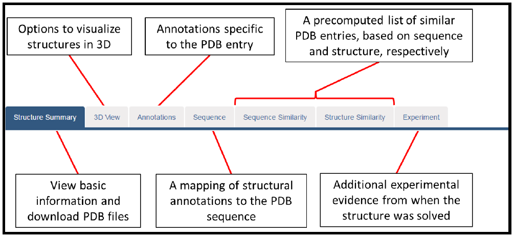
Before we begin, there is one additional feature of this page to look at – the navigation panel at the top of the page. This section of the page, shown below, can be quite easily overlooked, but it contains links to valuable information. In this overview we will only look at the “Structure summary” and “Sequence” tabs, but you are encouraged to have a look at the other tabs to see what information they display.
Basic information
This part of the page contains a quick summary of the PDB entry. In the top left hand corner of the page, images of the PDB 3D structure are shown. The right hand side of the page displays the PDB ID, as well as the name of the entry, describing what was solved. There is also additional information about the entry. In this example, we can see that this is a human protein, expressed in E. coli. The entry was also only made available in February of 2016.

Below this is the experimental overview of the entry. This gives an idea of the quality of the structure (for a full account of structure quality go to the Experimental Data & Validation section, further down the page). We can see this structure was solved by X-ray crystallography and as such has values for resolution, R-value and R-free. Ideally these values should be as low as possible for high quality structures. Resolution less than 3Å is acceptable, whereas 2Å and below is good. A good R-value is 0.2 or below and R-free should not be much higher than R-value. Authors at Proteopedia (http://proteopedia.org) suggest that R-free should not exceed resolution/10 by more than 0.5. For example, PDB entry 5F02 has a resolution of 1.43 Å, so R-free should not be much higher than 0.193. The value reported is 0.191, so we can safely assume the structure quality is fine.
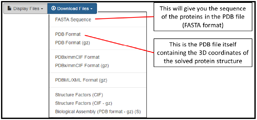
Additional structural validation data is also supplied by the wwPDB. Here values in blue indicate better quality, whereas those in red indicate poor quality. Finally, you can display or download the PDB entry by clicking on the dropdown menus in the top right corner of the page. This allows you to look at the PDB file or sequence and work with these on your local machine. Two of the download options are indicated below. Other file formats can be downloaded for a PDB structure, but these will not be used in the current protocol.
The literature segment
The literature section of the page contains information about where the PDB entry was published. It contains a link to the article in which this entry was published as well as a list of other PDB entries from this publication, as indicated below.

The macromolecules segment
This section of the page is important as it shows what proteins/nucleic acids are contained within the PDB entry. A PDB entry can consist of numerous chains, each representing a macromolecule. This page segment identifies the different proteins or nucleic acids found in the PDB entry, as well as the specific chains in the PDB file that they are represented by.
Below a feature breakdown of the protein, both at a sequence and structural level. In the screenshot, these are shown as follows. 1) Information from UniProtKB shows a representation of the full-length protein sequence and below this is the different domains that make up the protein. 2) PDB information for Cathepsin L is used to represent the known secondary structure of the protein and (3) shows the segment of the protein covered by this PDB entry specifically. A closer look at this mapping will show that only the heavy and light chains of Cathepsin L have been solved in this structure and the signal and activation peptides are not present.

Caution - know your protein
In the “molecular processing” section shown in (1) above, Cathepsin L is broken down into an activation peptide, Cathepsin L heavy chain and Cathepsin L light chain. In literature, these segments may go by different names. For example, the activation peptide is also known as the prodomain, which is cleaved before the protein is in its functional state, where only the mature domain remains. This domain is made up of the heavy and light chains indicated. It is important to know the protein you are working with in order to understand what is shown in the PDB
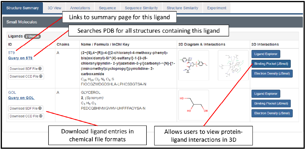
The small molecules segment
Here, the small molecules (not protein or nucleic acids, excluding water) are indicated. The PDB IDs of these ligands is shown (notice these are three letter codes), as well as the chains in which they are found. You can click on the ID of the ligand to go to its summary page and learn more about it, as well as find all structures in the PDB containing this ligand, as indicated.
One of the most useful features of this section is the Binding Pocket link. This allows you to look at the interactions between the ligand and the protein in an interactive 3D molecular viewer (JSmol). This can be used to look at how the ligand interacts with the protein, and which residues are involved in this interaction.
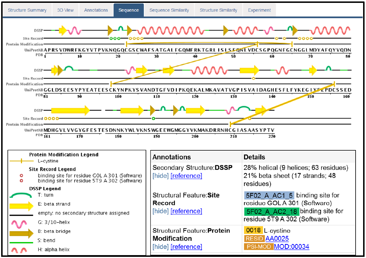
The sequence tab
One of the options in the navigational panel shown earlier on this protocol, was the Sequence tab. If you click on this tab, it will take you to the page shown below (you will need to scroll down a bit to view this segment of the page).
This provides a useful summary of the PDB entry, showing a mapping of secondary structure to the sequence. It also indicates additional sequence features, such as disulfide bonds formed between residues within the protein, as well as binding sites for the two ligands in this entry.
Final thoughts
This protocol was written to show how useful the PDB can be and what kind of information can be found about a protein structure. This was given as a basic overview and you are encouraged to explore this site to find additional information contained within.
Note, there is an additional resource provided by the PDB, PDB101 (http://pdb101.rcsb.org/). This is a great resource to learn more about the PDB, as well as structural biology.
Visualization of protein structures
AIMS:
Visualize protein structures in an online interactive molecular viewer
OBJECTIVES:
- Load PDB structure into an online molecular viewer
- Represent the sections of the PDB structure using different representations
EXPECTED OUTCOMES:
- To be able to produce a representation of a protein that highlights specific motifs or interaction site
PRIOR PROTOCOL(S) REQUIRED FOR THIS PROTOCOL:
Retrieval of PDB file from the Protein Data Bank or produce a protein model via homology modeling (See Protein Data Bank, HHPred, PRIMO sections)
SUGGESTED NEXT STEP(S):
There are no steps that follow visualization
Visualization of PDB files
Being able to visualize PDB files is useful for displaying your results in a way that looks appealing and helps you to better describe your work. Whether this involves displaying the interactions between a ligand and your protein or just displaying its different domains or binding pockets, visualization tools can be very useful.
Some of the most powerful and useful visualization tools can be downloaded onto your local machine and run locally. This protocol will focus on the web-based NGL Viewer, which can be found at http://proteinformatics.charite.de/ngl/html/ngl.html.
Go to the NGL Viewer website and upload your structure
The NGL Viewer is quite bare. After going to the site, click file, then either select the “Open” option to upload a file from your local computer or the “PDB” option to simple enter in a PDB ID as shown. In this we enter the PDB ID of Cathepsin L (5F02) into the search box and press the enter key.

NGL Viewer Overview
Before we continue, it is useful to note that when you go to the website, the first thing that is shown is a set of instructions showing how to use the viewer and also links to the documentation page for any additional queries.

At first glance
Once we have typed in the PDB ID and hit the Enter key, the NGL Viewer loads the structure, as shown below. By default it shows the protein in cartoon representation, colored by secondary structure. Non-water ligands are shown as sticks, whereas water molecules are shown as red spheres.
There is an options box on the right side of the screen that shows all representations for the PDB entry. Each of these representations can be filtered to apply only to specific residues (this is shown later) and an additional options set allows you to customize your selection.

Adding more representations
While the cartoon and licorice representations do look good, the NGL Viewer offers several other representation options. To see these click the button indicated in the screenshot below (it will be in the top right hand corner of your PDB entry), then select “Representation”. This gives a dropdown set with many different options. You can try these out to see which you like best.

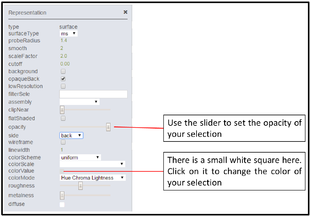
Customizing your selection
The options for customizing your selection are specific to each of the different representations, but there are two different options that are quite useful for beginners. These are indicated below for the surface representation. The first is opacity, which for the surface view, allows you to view other representations behind this view. The second is colorValue. It is not easy to see, but there is a small white square. If you click on it, you can select a color for your representation. This allows you to distinguish between different domains or motifs of your structure.
A simple example
When looking at structure 5F02 in the PDB (refer to Protein Data Bank protocol), we can see that this contains the light and heavy chains of the Cathepsin L mature domain, residues 1-175 and 177-220 in the PDB structure, respectively. In the example below, we created two cartoon selections and two surface representations. Next, we entered in the residue ranges for the two subdomains into the filter boxes. These were then colored green for the heavy chain and blue for the light chain. The ligands in the structure are numbered 301 and 302. To show these, a ball-and-stick representation was created and filtered by these residue numbers.
The result of this is shown below. A zoomed in view of the drug molecule 5T9 as it is bound in to Cathepsin L.

Final thoughts
This protocol gives a quick overview of one web-based protein visualization tool. Essentially all visualization tools work in a similar manner. It just takes a few minutes of playing around with the options to produce the results you want.
Note, there are more useful protein visualization tools that can be used on your local machine. A good example is PyMOL, which allows you to take high quality images of protein structures, display protein-ligand interactions and label residues, among other things. If you can download this and install it on your PC, you will find it very useful.
Homology detection & structure prediction (HHpred)
AIMS:
Explore the use of web-based homology modeling servers such as HHpred in acquiring 3-Dimensional (3D) protein structures for protein targets where no such structures exist.
OBJECTIVES:
- Use HHblits to identify distant or close structural homologs
- Select suitable templates for homology modeling
- Use HHpred to model proteins (SERA2)
- Analyze the results
EXPECTED OUTCOMES:
- Produce 3D structural models of the target proteins
- Understand the role of HHpred and homology modeling in protein analysis
PRIOR PROTOCOL(S) REQUIRED FOR THIS PROTOCOL:
Retrieval of protein sequences (See, NCBI, MSA and BLAST sections) and the PDB protocol
SUGGESTED NEXT STEP(S):
Ligand and protein interaction
INTRODUCTION:
Cysteine proteases are essential in hemoglobin metabolism and survival of the malaria parasite. The best characterized of these are falcipains1. They are made up of a four papain enzyme family, and Falcipain-2 and Falcipain-3 have been extensively studied as potential drug targets. Serine repeat antigens (SERAs) carry cysteine protease motifs and disruption studies have shown that members of this family such as SERA-5 and SERA-6 are essential to the parasite2. In this exercise we propose to explore SERA-2 and SERA 8, members of the SERA family. Their crystal structures have not yet been resolved. This protocol will guide you on how to use the HHpred3 web-server (https://toolkit.tuebingen.mpg.de/HHpred) to produce models for these protein targets.
BEFORE WE BEGIN: What is homology modeling?
Homology modeling also known as comparative modeling or template based modeling (TBM) of proteins, refers to the modeling of a protein 3D structure where none exists by using a template(s) based on known experimentally determined homologous proteins. This is possible due to evolutionary conservation of across related proteins. Proteins related through evolution are shown to have similar sequences i.e. homologs. Furthermore, the three dimensional protein structures of naturally occurring homologous proteins have been observed to be more conserved than their protein sequences.4 HHpred like several other modeling engines uses MODELLER (https://salilab.org/modeller/) for homology modeling.5, 6, 7, 8
1. Rosenthal, P. J. (2011). Falcipains and other cysteine proteases of malaria parasites. In Cysteine Proteases of Pathogenic Organisms (pp. 30-48). Springer US.
2. Huang, X., Liew, K., Natalang, O., Siau, A., & Zhang, N. (2013). The Role of Serine-Type Serine Repeat Antigen in Plasmodium yoelii Blood Stage.
3. Söding, J., Biegert, A., & Lupas, A. N. (2005). The HHpred interactive server for protein homology detection and structure prediction. Nucleic acids research, 33(suppl 2), W244-W248.
4. Kaczanowski, S., & Zielenkiewicz, P. (2010). Why similar protein sequences encode similar three-dimensional structures?. Theoretical Chemistry Accounts, 125(3-6), 643-650.
5. A. Sali & T.L. Blundell. Comparative protein modelling by satisfaction of spatial restraints. J. Mol. Biol. 234, 779-815, 1993.
6. A. Fiser, R.K. Do, & A. Sali. Modeling of loops in protein structures, Protein Science 9. 1753-1773, 2000.
7. M.A. Marti-Renom, A. Stuart, A. Fiser, R. Sánchez, F. Melo, A. Sali. Comparative protein structure modeling of genes and genomes. Annu. Rev. Biophys. Biomol. Struct. 29, 291-325, 2000.
8. B. Webb, A. Sali. Comparative Protein Structure Modeling Using Modeller. Current Protocols in Bioinformatics, John Wiley & Sons, Inc., 5.6.1-5.6.32, 2014.
STEP ONE: QUERY SUBMISSION
Protein targets
Example: SERA2 (GenBank accession number: SBT75712.1, name: serine-repeat antigen, putative [Plasmodium falciparum]).
Exercise: SERA8 (NCBI Reference Sequence: XP_001349583.1, name: serine repeat antigen 8 (SERA-8) [Plasmodium falciparum 3D7]).
Protein sequence retrieval and submission of queries to HHpred
Retrieve the protein sequence in FASTA format using the accession number provided as described in the prior protocols (http://www.ncbi.nlm.nih.gov/). Go to the HHpred web-server (https://toolkit.tuebingen.mpg.de/hhpred) and submit the query sequence into the input text box as shown in Figure 1.

HINT: This particular step can take in excess of 15 minutes, optional inputs include a Job-ID and an email address where notifications can be sent once the job is completed. You have the option to use HHblits9 or PSIBLAST10 for your homology search, try both and compare the results. Are the top hits the same?
9. Söding J. (2005) Protein homology detection by HMM-HMM comparison. Bioinformatics 21: 951-960. PMID: 15531603
10. Altschul, Stephen F., et al. "Gapped BLAST and PSI-BLAST: a new generation of protein database search programs." Nucleic acids research 25.17 (1997): 3389-3402.
STEP TWO: SEARCHING FOR DISTANT OR CLOSE HOMOLOGS
Analyzing the results of the homology search
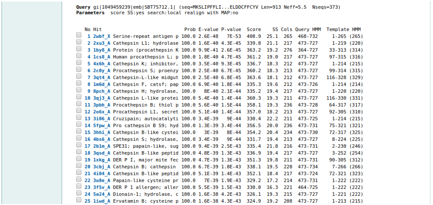
The HHpred homology search results are organized into three sections, a colored bar-graph, a table, and pairwise alignments. The search results for SERA2 are shown in Figure 2 (a, b and c)
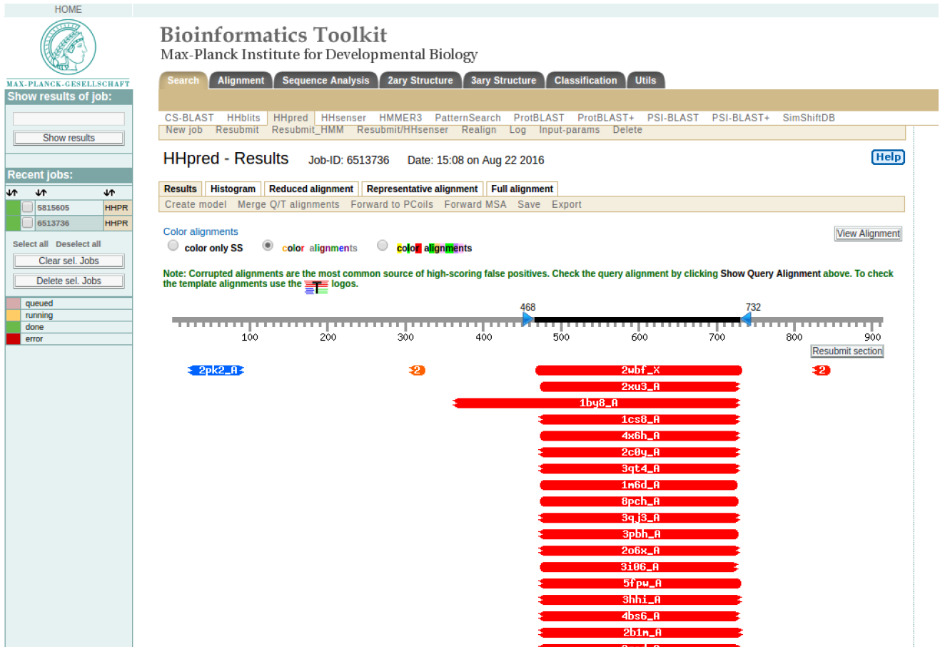
HINT: What does the color coding tell you? Can you comment on the coverage of the templates against the target sequence?
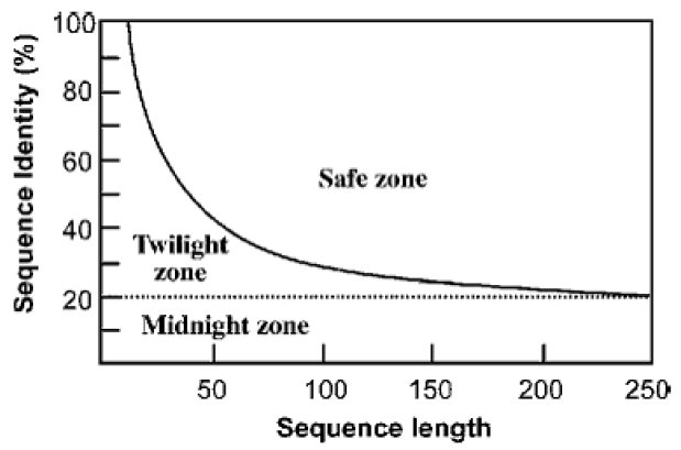
HINT: When making inferences about sequence identity, it is very important to consider the length of your target sequence.
For example, here is a homology relationship of two protein sequences. If both were 150 residues long and their sequence identity was 30% this would fall in the safe zone. However if they were both 25 residues long, and had a sequence identity of 60% this would fall in the twilight zone, that is described as a mixture of actual homologs and randomly related sequences.11
Can you comment on the E-values and the proportion of your hit sequence(s) that aligns with your target protein i.e. ‘coverage’. Does it matter whether the hits are from the same phylogenetic sub-family as your query sequence? How does SERA2 compare to SERA8? Please note these results.
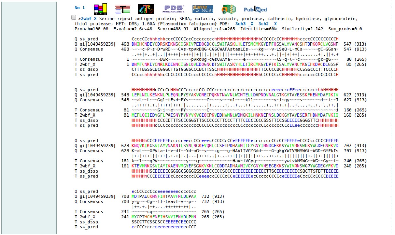
HINT: Can you please comment on secondary structure prediction alignment? (‘cccccc’, ‘hhhh’..etc). Also please note the resolution of your top crystal structures. Above the alignment are links to for example: the Protein Data Bank (PDB) and PubMed for related articles on the hit.
11. Rost, B. (1999). Twilight zone of protein sequence alignments. Protein engineering, 12(2), 85-94.
STEP THREE: HOMOLOGY MODELING
Template selection
Selection of proper templates for homology modeling depends on several factors. These include: the resolution of the template, the template environment (mutations, pH, presence/absence of ligands), biological function, sequence coverage, % sequence identity, the family of proteins (phylogenetic analysis can be helpful in identifying the closest subfamily groups) or even whether to use single or multiple templates. For more information on template selection see here https://salilab.org/modeller/tutorial/ or http://tinyurl.com/hs6kq55
The initial homology search was to identify suitable structural templates. To create a model click on the create model tab as show in Figure 3 (a). For this particular exercise we shall use the ‘Automatically select best templates’ option.
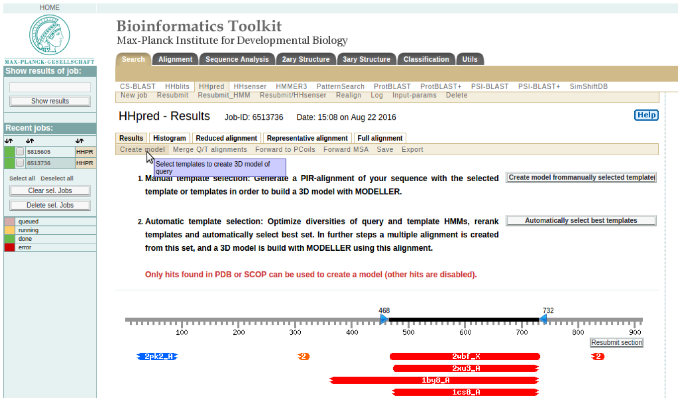
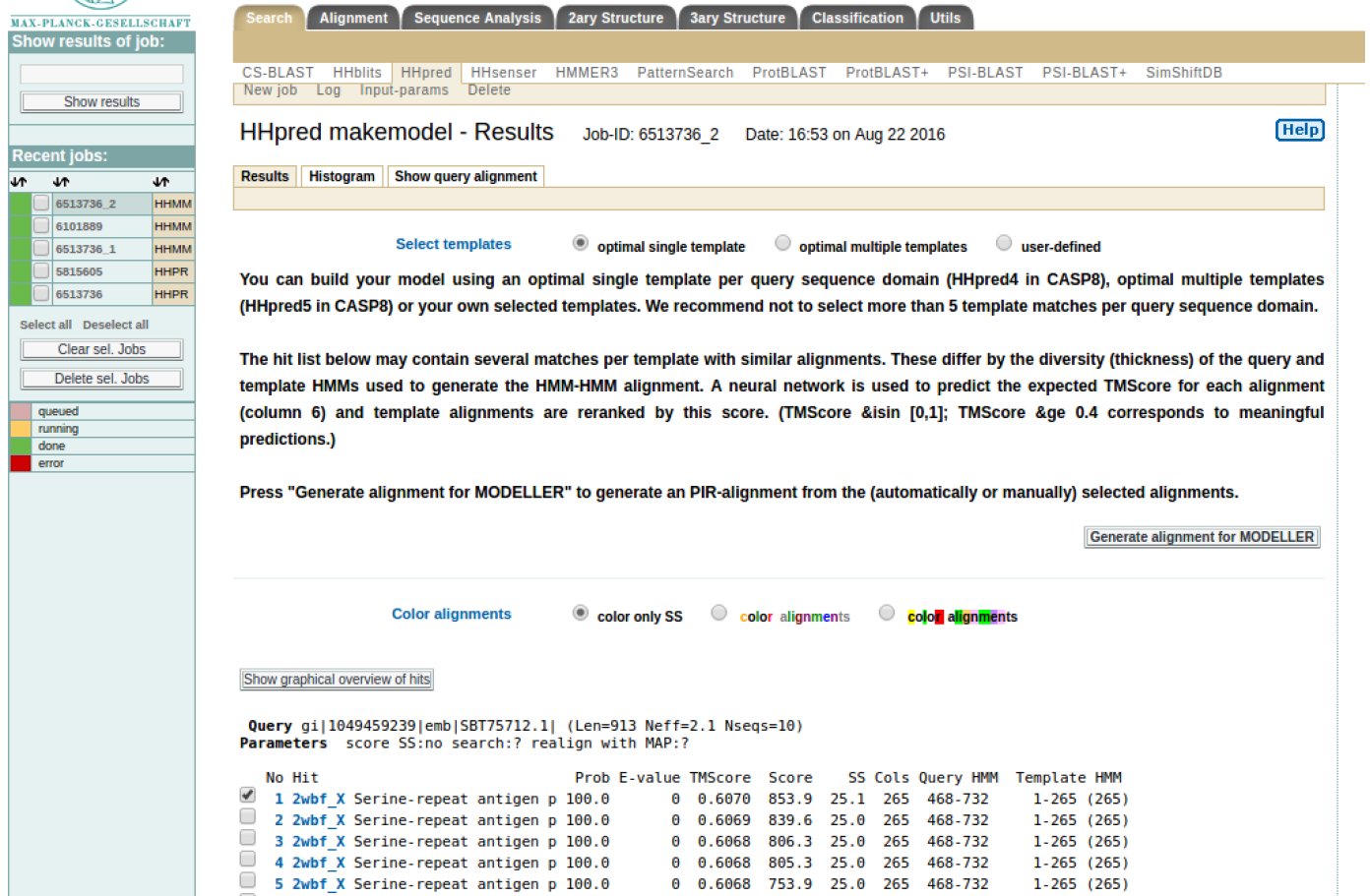
HINT: It should take around 5 minutes to generate the result as shown in Figure 3 (b) where the best template is automatically checked.
HINT: Please note the residues in your query sequence that align with the template (for example in SERA2 above, it aligns with template 2wbf_X from sequence residue 468 to 732). Click “Generate alignment for MODELLER”. It will generate a result that is shown in Figure 3 (c).
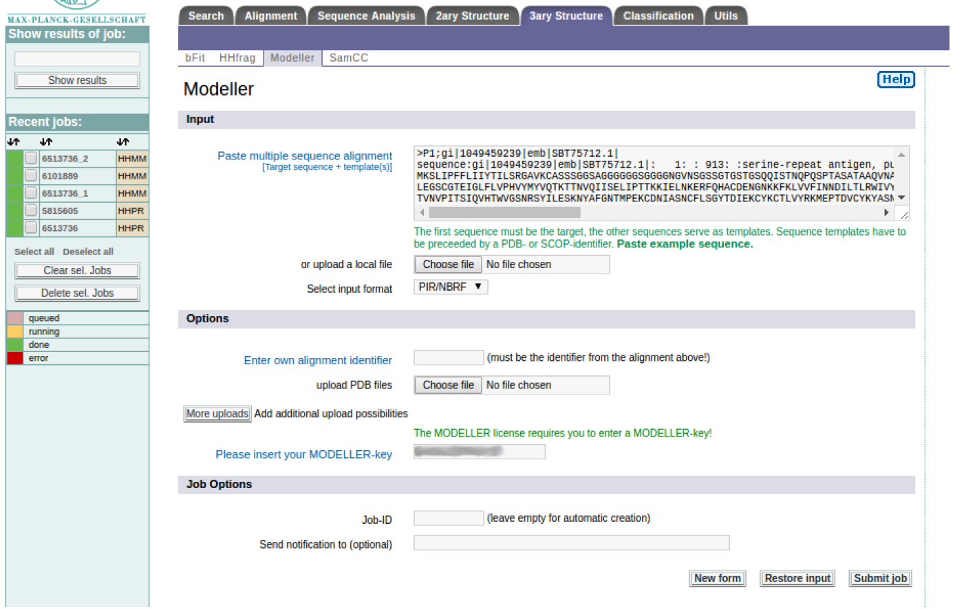
HINT: A key for MODELLER can be obtained from their website. In the input text box is the alignment of the query sequence and template in the PIR format. At this stage click “Submit job” to initiated homology modeling.
STEP FOUR: HOMOLOGY MODELING RESULTS AND EVALUATION
MODELLER results
The modeling results consist of a PDB file computed by MODELLER, Figure 4 (a). Other useful tabs include “View 3D structure” that allows you to visualize the protein 3D structure using a Java applet called Chemis3D, Figure 4 (b). It also includes tabs of useful graphical tools for evaluating the quality of your model such as ‘Model quality VERIFY3D”, Figure 4 (c), “Model quality SOLVX”, and “Model quality ANOLEA”, Figure 4 (d).12, 13, 14, 15 Please click on the HELP button for a more detailed overview of the results.
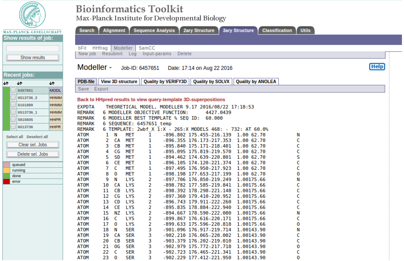
HINT: You can copy the PDB file into a text editor and save it to your desktop if you want to view the structure on your computer later (save it with the file extension ‘.pdb’)
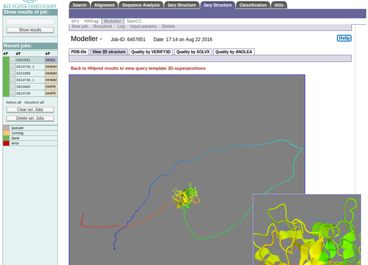
HINT: You can zoom into and rotate the model using this viewer. Visually analyze the structure, for example are there any knots? Can you comment on the long loops?
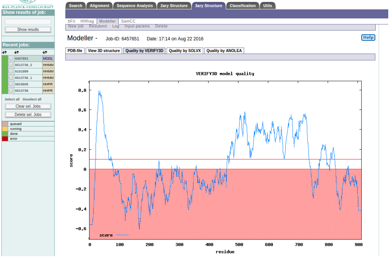
HINT: The regions below the red line are generally poorly modeled. How does this compare to the alignment and model visualisation?
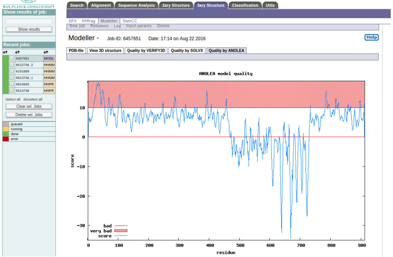
HINT: Both VERIFY3D and ANOLEA show that the poorly modeled regions are 0-468 and 732-900 residues, what could be the possible reason? Appreciating this will help you understand the limitations of homology modeling. Congratulations you have made a structural model for part of the SERA2 protein, how can you improve the modeling result?
EXERCISE:
Follow the same procedure and create a structural model for SERA8.
12. Eisenberg, D., Lüthy, R., & Bowie, J. U. (1997). [20] VERIFY3D: Assessment of protein models with three-dimensional profiles. Methods in enzymology, 277, 396-404.
13. Holm, L., & Sander, C. (1992). Evaluation of protein models by atomic solvation preference. Journal of molecular biology, 225(1), 93-105.
14. Melo, F., Devos, D., Depiereux, E., & Feytmans, E. (1997, June). ANOLEA: a www server to assess protein structures. In ISMB (Vol. 5, pp. 187-190).
15. Melo, F., & Sali, A. (2007). Fold assessment for comparative protein structure modeling. Protein Science, 16(11), 2412-2426.
Protein interactive modeling - PRIMO
AIMS:
Use PRIMO to model the structure of a protein given only its sequence.
OBJECTIVES:
- Identify suitable homologs to be used as templates
- Align target sequence with selected templates
- Produce models of your protein
- Evaluate the quality of your models
EXPECTED OUTCOMES:
- To be able to use PRIMO to produce models of a protein structure
- To understand which tools to use for homolog detection in a given scenario
- To understand which alignment tools to use in a given scenario
- To be able to trim your alignment when necessary
- To be able to evaluate your produced models
PRIOR PROTOCOL(S) REQUIRED FOR THIS PROTOCOL:
Retrieval of homolog structures (see NCBI, BLAST, and HHPRED protocols), PDB, and Multiple Sequence Alignment.
SUGGESTED NEXT STEP(S):
Visualize protein models in 3D (see Visualization protocol) and calculate ligand interactions (see Ligand Interaction protocol)
BACKGROUND:
Homology modeling, also called comparative modeling, refers to the practice of constructing an atomic resolution, three-dimensional model of a "target" protein based on the known structure of a homologous protein, referred to as a "template". Homology modeling relies on the idea that protein structure is more conserved than the underlying protein sequence. As such, proteins can be modelled using homologs with sequence identity as low as 30%.
Homology modeling follows a four step process (Fig. 1):
- Template identification;
- Target-template alignment;
- Model construction; and
- Model assessment
During the template identification step, the target protein sequence is provided as input to programs such as Protein BLAST, HHSearch, HMMER, and CMSearch in order to identify homologous proteins. These homologous proteins are used as templates when constructing the model of the target protein. As such, it is important to select good quality templates that cover as much of the target protein as possible. If a template doesn't cover the whole protein sequence, additional templates can be selected that cover the missing regions. Homologs that are selected to be used for modeling are referred to as “templates”.
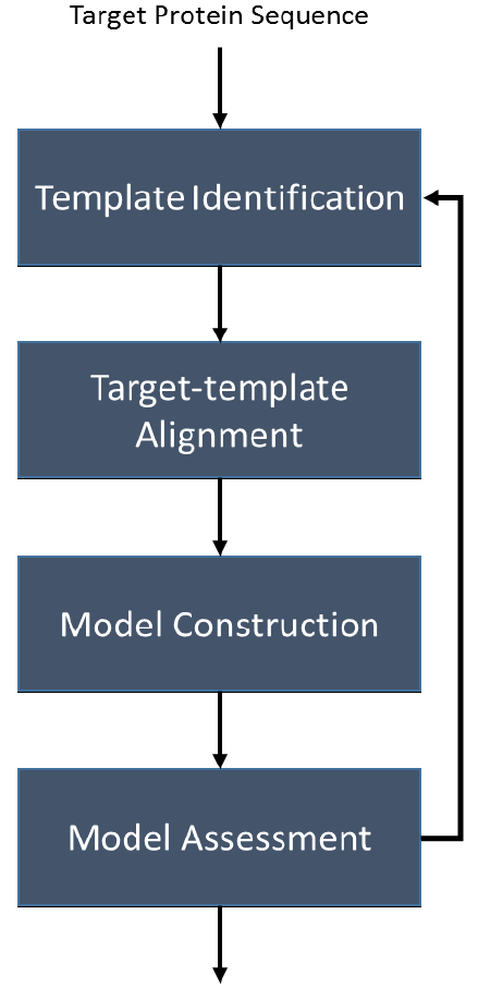

During the target-template alignment stage, templates identified in the previous stage are aligned to the target sequence. The alignment maps residues in the target sequence to residues in the template sequences, so that structural information from these regions of the templates can be copied to the target.
During the modeling stage, the templates identified in step 1 and the alignment produced in step 2 are used to produce models of the target protein. Structural information from the templates is mapped to the target based on the target-template alignment.
Once a model of the target protein has been produced, it needs to be assessed to determine its accuracy. Online tools such as PROSA, ANOLEA, and Verify3D can be used for this. Depending on whether a good quality model has been produced or not, the previous steps can be repeated to improve the quality e.g. by selecting alternative templates or editing the alignment.
Various online tools exist that perform homology modeling. This protocol will teach modeling using PRIMO, an interactive homology modeling platform that allows users to select different tools and alter various parameters to improve the quality of their models. PRIMO can be accessed at https://primo.rubi.ru.ac.za.
PRIMO:
Introduction
PRIMO is a homology modeling platform that walks the user through each step in the homology modeling process. It lets the users select which tools they want to use at each step and allows them to modify modeling parameters. As such, PRIMO provides more control over the homology modeling process than most online tools and is useful for educational purposes. What follows is a guide to using PRIMO.
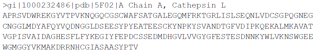
EXAMPLE DATA:
For the purpose of this tutorial, we will be modeling Cathepsin L, which has the following protein sequence:
USER ACCOUNT CREATION:
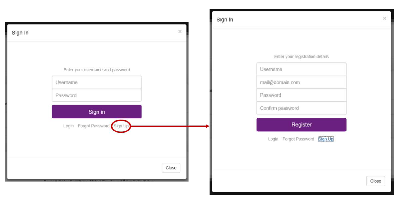
In order to use PRIMO, users must first create an account on the site. To do this, the user must click on the green “power” button in the top-right of the PRIMO interface. A dialog box asking the user to sign in will appear. To create an account, the “Sign Up” link, which can be found below the “Sign In” button must be clicked (Fig. 2A). This provides the user with an interface to create a new account (Fig. 2B). Here, the user should enter a unique username, their e-mail address, and a secure password, before clicking on the “Register” button to create the account.
STARTING A JOB:
PRIMO provides a user-friendly, initial input page (Fig. 3), where, at a minimum, the user must provide a job name, the MODELLER key, and a target protein sequence – all these fields are located in the “Required input” box. (Fig. 3A)
The job name can be anything the user desires. Preferably, this name will be something that easily distinguishes the job from other jobs that the user has run, making it easy to identify later on.
PRIMO uses software called MODELLER to perform the actual model construction. This software requires a license key to run. To obtain the MODELLER key, click the link next to the input field to go to the MODELLER website and follow the instructions provided there. Once the key has been obtained, it should be entered into the provided field. After the user runs their first job, the key will be saved to their user profile. As such, this field will be automatically populated in future.
The most important piece of input is the actual target sequence that will be modelled. This should be entered into the text area provided.
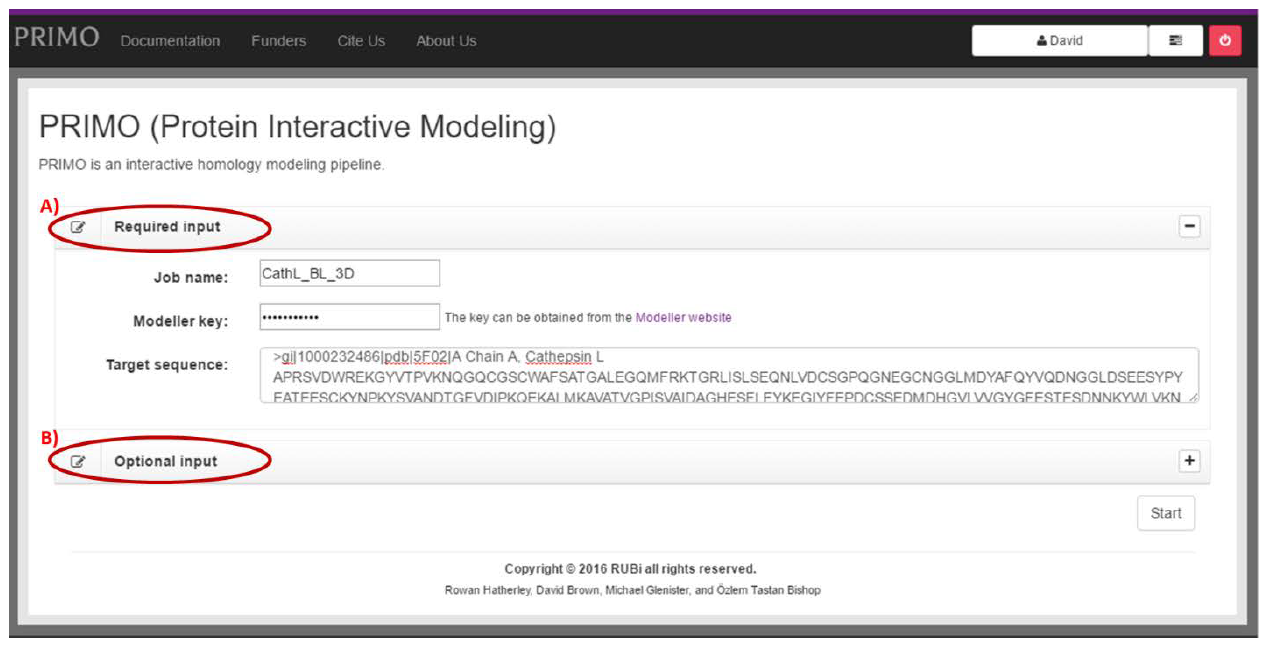
Below the “Required input” box, is the “Optional input” box (Fig. 3B). This box can be expanded by clicking the “plus” (+) in the right corner of the box. This will provide the user with a number of additional input options (Fig. 4), which are either optional or already have default values entered into them. Table 1 provides a summary of the fields.
| Field | Option | Description |
|---|---|---|
| Job Description | - | A user-input description that gives context to the job. |
| Email notifications | - | When enabled, e-mails will be sent to the user whenever their job requires attention. |
| Template identification | Automatically identify templates | Automatically identify templates |
| Specify templates | Specify templates via their PDB ID and chain in the format PDBID:CHAIN e.g. 5F02:A. | |
| Upload own templates | Upload PDB files and specify which chains to use as templates. | |
| Alignment | T-COFFEE | Use T-COFFEE to align. Users have the option of running T-COFFEE in standard mode or 3D-Coffee mode. The latter takes protein structure into account when aligning. |
| MAFFT | Use MAFFT to align. Users have the option of running MAFFT in standard mode or Psuedo-homologs mode. The latter identifies similar sequences and performs a multiple sequence alignment to improve accuracy. | |
| MUSCLE | Use MUSCLE to align. | |
| CLUSTAL-O | Use CLUSTAL Omega to align. | |
| BLAST/HHSearch | If BLAST was used to identify templates, use the BLAST alignment. If HHSearch was used to identify templates, use the HHSearch alignment. | |
| Modeling | Model prefix | Models that are produced will start with this prefix |
| No. of models | The number of models that will be produced. | |
| Refinement method | The level of refinement to use when constructing models. Slower levels generally produce more accurate models. |
In the example shown in Fig. 4, we have selected to identify templates using BLAST and align using 3D-Coffee. As such, we have entered in a relevant description of the job in the “Job description” field. BLAST was selected, because closely related homologs with known structures in the PDB exist for Cathepsin L (as will be shown later in the BLAST results). When it comes to identifying highly similar homologs, BLAST produces superior results to HHSearch. In addition, it also runs much faster, and as such, it is always useful to BLAST for templates first. If no suitable templates are found, you can try again using HHSearch. HHSearch produces superior results when identifying distantly related homologs. However, HHSearch can sometimes take around fifteen minutes to complete, depending on the length of the target sequence.
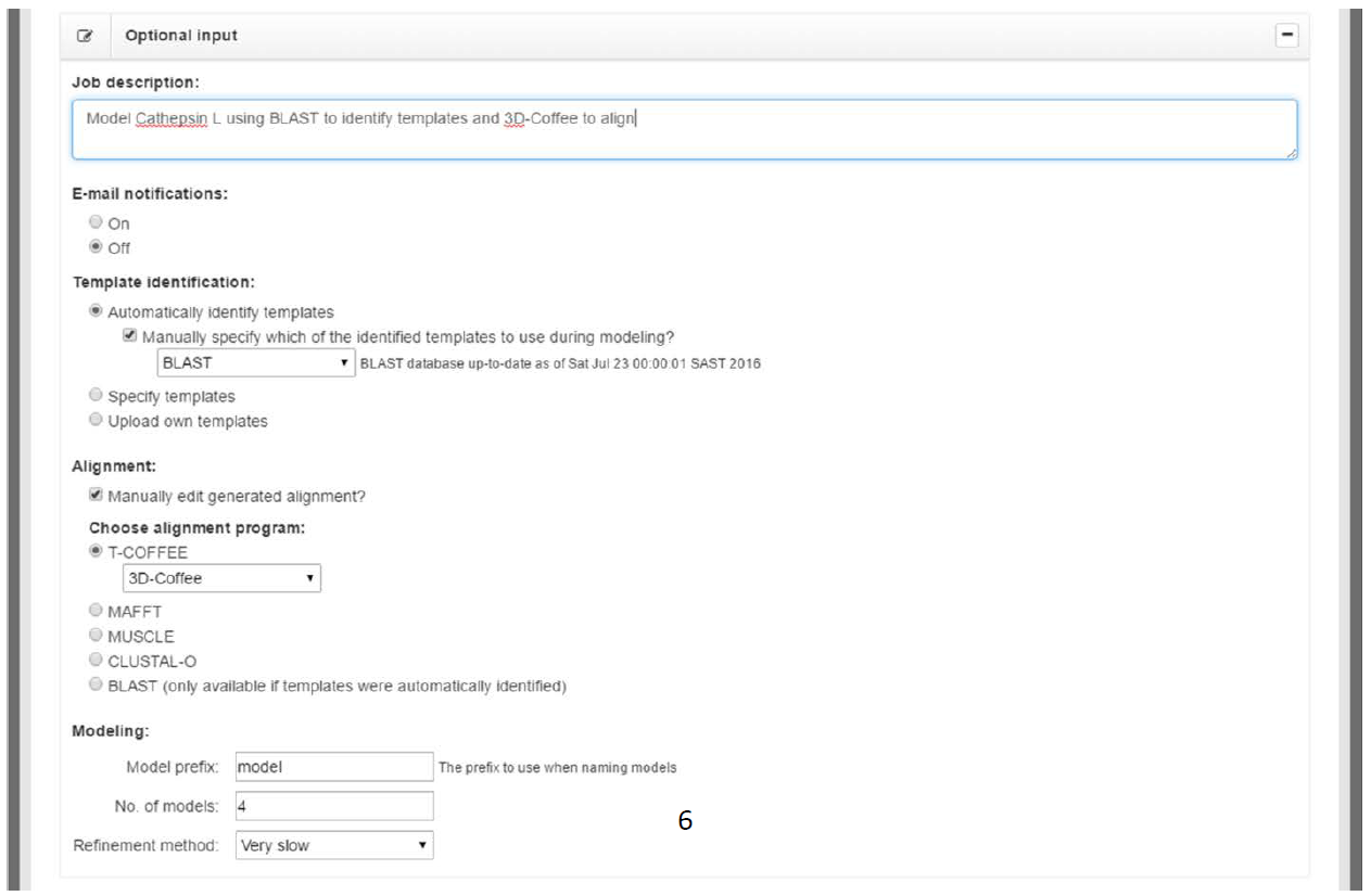
In addition, the checkbox labeled “Manually specify which of the identified templates to use during modeling?” is checked. Having this checkbox checked tells PRIMO to pause once potential templates have been identified and let the user select one or more templates to move forward with. If it were unchecked, PRIMO would automatically select the highest ranked template according to the BLAST/HHSearch results. The highest ranked template may not necessarily be the best template, however.
Similarly, the “Manually edit generated alignment?” checkbox tells PRIMO to pause after the alignment stage and let the user edit the alignment. Alignment programs are not perfect and, as such, manually editing the alignment is sometimes necessary. This is especially true for distantly related proteins
In Fig. 4, we have selected to align using T-COFFEE in 3D-Coffee mode. 3D-Coffee takes into account structural information when aligning sequences. This is important for homology modeling. Structural alignments also produce the most pronounced benefits when aligning highly divergent sequences. That being said, it is useful to try different alignment methods as there is no method that consistently outperforms other methods.
The last section on this page is the “Modeling” section. Here we can enter a prefix for our models, select how many models will be produced, and select the refinement method. The prefix option is simply used to provide unique names to models across different jobs. The latter two parameters allow the user to adjust to improve either speed or accuracy. Increasing the number of models produced increases the chance of producing better models, while decreasing the speed that the job will be completed in. Similarly, using slower refinement levels improves accuracy at the cost of speed.
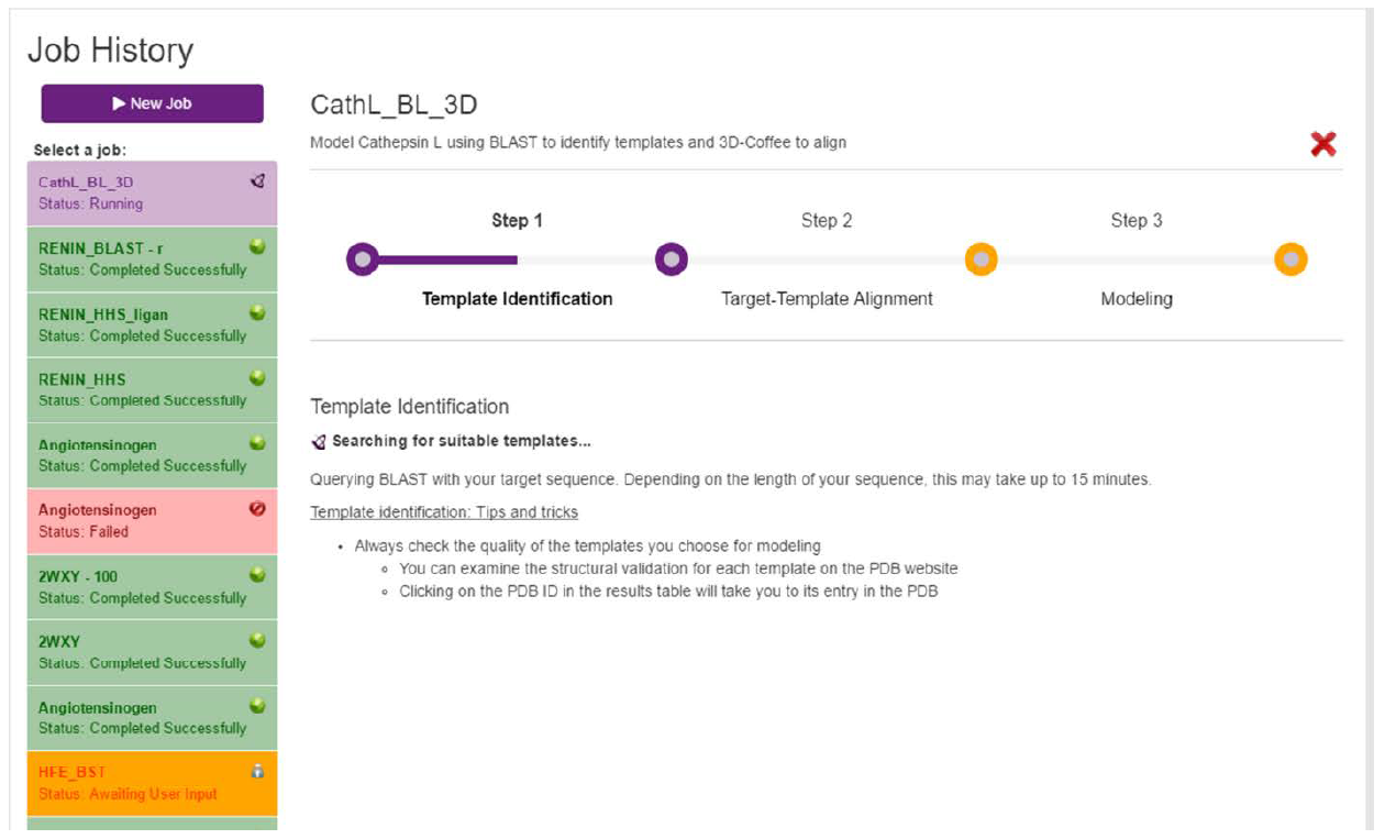
Once the user is happy with their choices, they can run the job by clicking the “Start” button in the bottom-right corner. This will start the modeling process and take the user to the loading page illustrated in Fig. 5.
TEMPLATE SELECTION:
Regardless of whether BLAST or HHSearch is run, a list of templates will be returned and displayed in a table (Fig. 6). The first column in this table displays the PDB ID of the structure and links to the structure at the PDB website. The second column displays the chain in the structure that matched the target sequence.
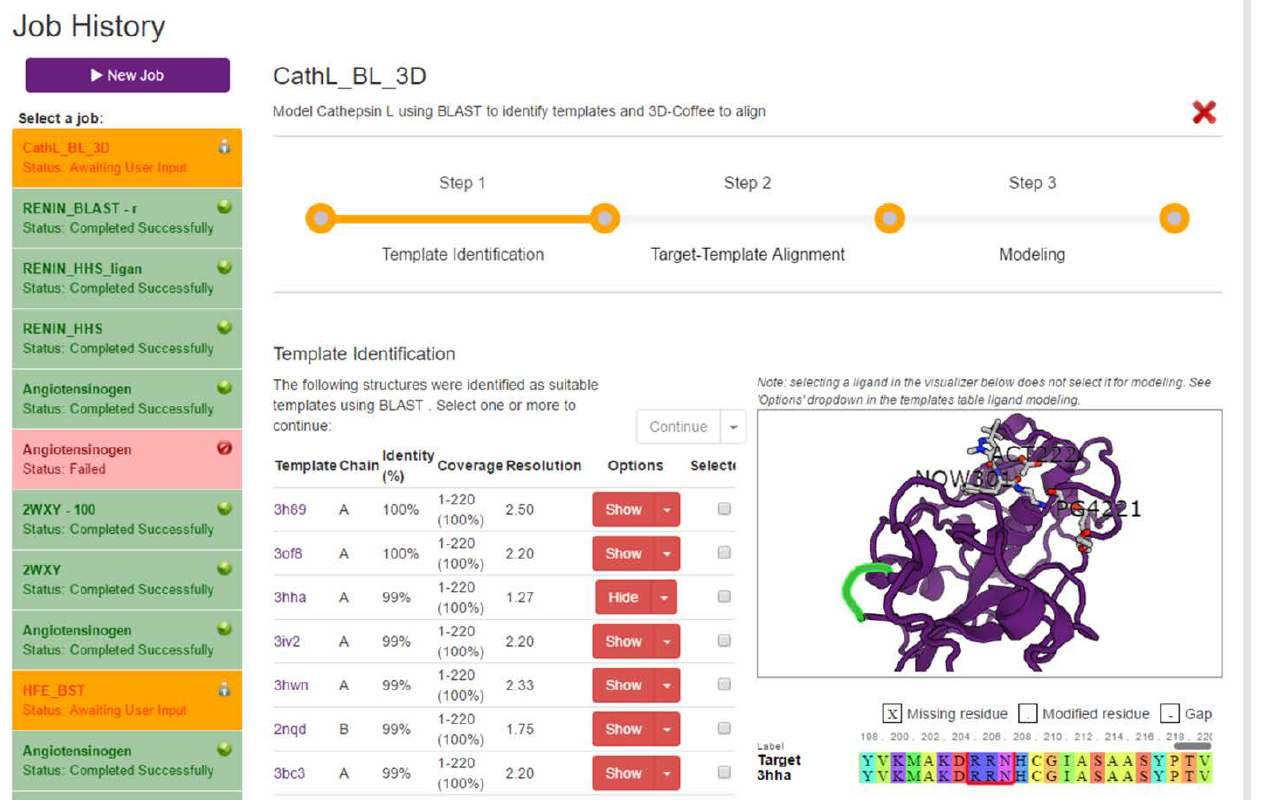
The third and fourth columns display the sequence identity and coverage, respectively. Sequence identity refers to how similar the target sequence is to the template sequence, while query coverage refers to the portion of the target sequence that is covered by the template sequence.
The resolution of the structure is displayed in the fourth column. A lower number here means a higher (better) resolution. For homology modeling, we are usually happy with anything under 2.5 Angstroms.
The options column provides the user with two options. Firstly, the user can click the “Show” button to display the structure on the right of the screen. Secondly, clicking on the little dropdown arrow on the right of the button will bring up a second menu, which has the option “Select ligand”. This lets users select the ligands they wish to include in their models.
The last column is where the user selects which homologs to use as templates when modeling. Clicking one of the checkboxes will select that homolog. When selecting homologs, the quality of the structure is very important. By following the link to the PDB, one can assess whether the structure quality is decent (see PDB protocol). Resolution is should also be taken into account for this. High query coverage is also important. Regions of the target that aren’t covered by the templates cannot be reliably modelled. A higher sequence identity can also improve results (not always), but homology modeling can still be performed reliably with low sequence identity.
Based on the above, 3HHA appears to be the best template returned by BLAST. At 1.27 Angstroms, it has very high resolution, it covers 100% of the target sequence with a sequence identity of 99%, and checking the PDB shows that it is a good quality structure. As such, we will select this homolog as our template. The homolog is selected by clicking on the checkbox in the last column of the templates table.
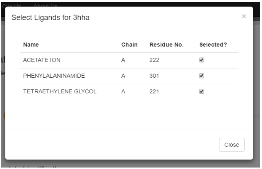
Once we have selected the ligands, we can close the dialog and continue our modeling job. In the next step, the chosen template will be aligned to the target sequence.
TARGET-TEMPLATE ALIGNMENT
In the previous step, we selected a template (3HHA) and the three ligands in that template. To align the template to our sequence, we need to continue on to the next stage. There are two ways to achieve this.
Firstly, we can align the using the option we selected in the initial input page (T-COFFEE in 3D-Coffee mode, manually edit the alignment) simply by clicking the “Continue” button, located above the templates table. This will immediately start aligning your target sequence with your selected templates. Please note, if you have not selected a template, this button will be disabled.
The second option is to click on “Edit and continue”, which can be found by selecting the little arrow next to the “Continue” button. This will bring up a dialog (Fig. 8) that allows you to change the alignment options you chose on the initial input page. Once you have updated your alignment options, clicking on the purple “Continue” button at the bottom of the dialog will start the alignment process.
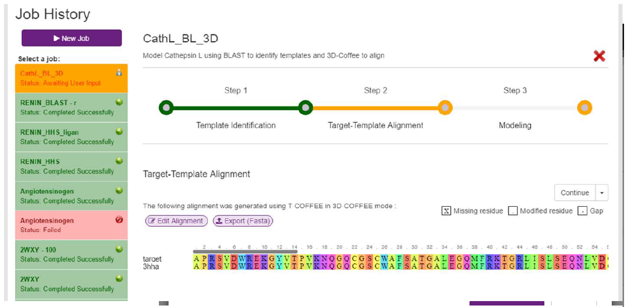
Alignment options before aligning your target and templates
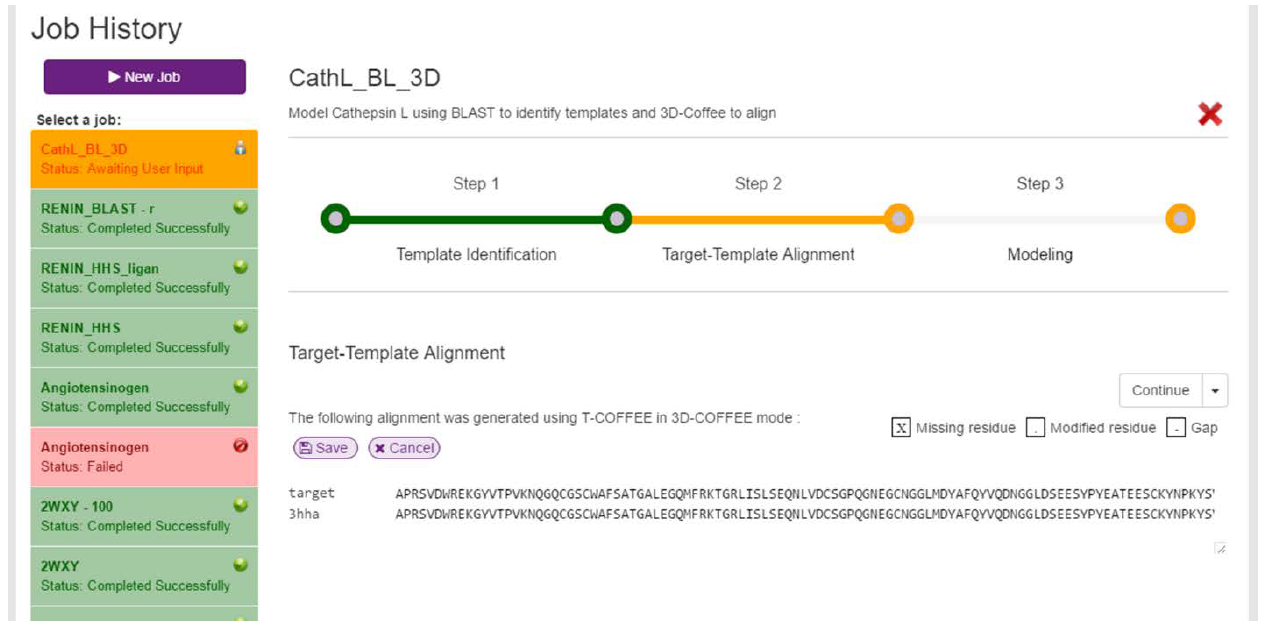
After clicking continue, a loading screen similar to the one illustrated in Fig. 5 will be displayed. Once the target and template have been aligned, the resulting alignment will be returned and displayed (Fig. 9). On this screen, the user can edit the alignment by clicking on the purple “Edit Alignment” button. If clicked, the alignment will be made editable in a text area (Fig. 10). The target sequence can be edited in any way, but there are limitations on how the templates can be edited. Templates can only be trimmed from the outside i.e. Gaps cannot be created between the C- and N-terminals. If the user attempts this, an appropriate error message will be displayed when the user tries to save the edits.
In our example, 3D-Coffee has produced a perfect alignment, which doesn’t need to be edited. As such, we can move on to the modelling stage.
MODEL CONSTRUCTION:
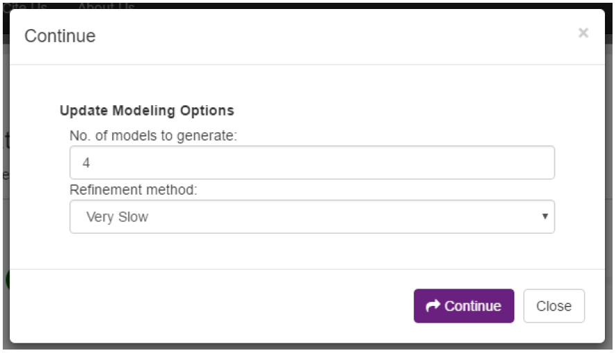
On the alignment page, we can click on the “Continue” button to move on to the modeling stage. Like we showed after the template identification stage, we can also click on the “Edit and continue” button to update the modeling parameters (Fig. 11) we set on the initial start page. For the sake of this tutorial, our initial parameters are fine and we will continue with them.
As with the previous stages, clicking on the “Continue” button will present the user with a loading screen and move the progress bar forward. When the job completes, the models are returned to the user (Fig. 12). The models are listed in a table made up of five columns.
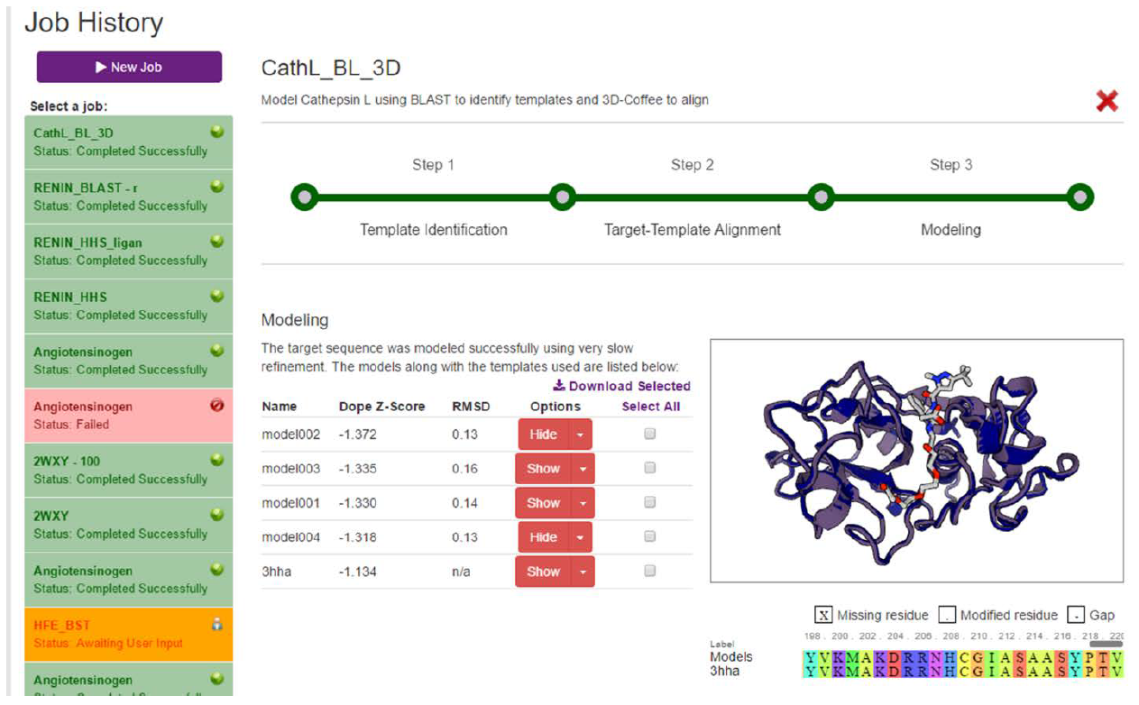
The first column contains the name of the model. Notice that the models are named using the prefix we chose on the initial page.
The second column contains the DOPE Z-Score, a metric for the overall quality of the model. As DOPE is a global score, it cannot tell you whether there are local regions of the protein that have not been modeled well. It is quick to calculate, however, and is a good way to weed out the really bad models. When judging quality using the DOPE Z-Score, we are looking for scores less than -0.5, but preferably approaching -1. As we can see in our example, our top model has a DOPE Z-Score of -1.372. This is a very good score and is even an improvement over the template’s score.
The RMSD column is a measure of how different the backbone of our models are when compared to the templates that were used to model them. This is generally not that useful a metric as it does not consider sidechains.
The Options column allows us to visualizes our models by clicking on the “Show” button. We can superpose our models over each other as well as the template by clicking on the various “Show” buttons. The little dropdown button on the right of the “Show” button reveals a “Structure Evaluation” button, which we will talk more on in the next section.
The last column allows users to select and download the models and templates. Users can select only the models they want or use the “Select All” link to download everything.
MODEL EVALUATION:
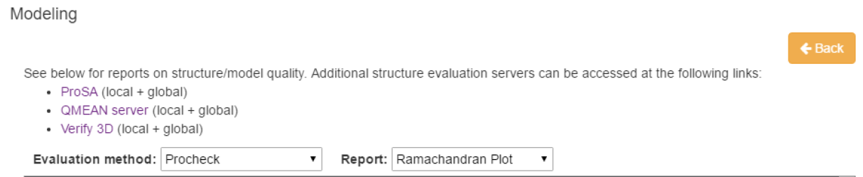
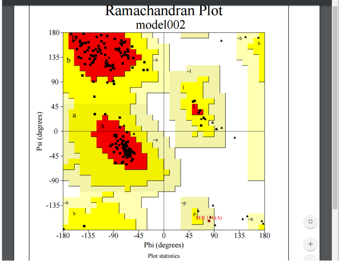
We have already covered evaluation using DOPE Z-Score and RMSD, but PRIMO also provides local evaluation via PROCHECK. To evaluate using PROCHECK, select the dropdown button in the Options column and click the “Structure Evaluation” button. The model will now be evaluated using PROCHECK. The resulting evaluation for model002 is displayed in Fig. 13.
PROCHECK produces a number of graphs depicting model quality. These graphs can be viewed by selecting them in the Report dropdown and include:
- Ramachandaran plot
- Ramachandaran plots for all residue types
- Chi1-Chi2 plots
- Main chain parameters
- Side-chain parameters
- Residue properties
- Main-chain bond lengths
- Main-chain bond angles
- RMS distances from planarity
- Distorted geometry
This page also links to other model evaluation servers including ProSA, QMEAN, and Verify 3D. To be sure you have a good quality model, you should use as many evaluation methods as possible.
REPEATING JOBS:
Jobs can be repeated from any stage at any point. By clicking on the nodes in the progress bar, you can go back to template identification stage and select different templates or change the alignment options, before clicking on “Continue” again to repeat the job. Similarly, you could go back to the target-template alignment stage and edit the alignment or change the modeling parameters. This functionality is very useful if you want to test a number of different templates or try out different alignment programs to see which one will produce the best alignment. After clicking “Continue”, the user can immediately go back to the previous stage, change parameters, and repeat the job with a different template, alignment method, or both. As such, the user could have a number of jobs running in parallel and select the best alignment to go forward with at the next stage.
SUMMARY:
Homology modeling is useful when the structure of a protein has not been solved experimentally via techniques such as X-ray crystallography or NMR. Homology models offer an alternative means of studying a protein’s structure, generating hypotheses about the protein’s function, and directing further experimental work.
The homology modeling process consists of four important steps. The first is the identification of suitable templates. Tools such as BLAST and HHSearch can be used for this. BLAST is a quick method that is good at identifying potential templates that are closely related to the target protein. HHSearch, on the other hand, can identify distantly related homologs, but takes longer to run and is not so adept at identifying more closely related sequences.
Once suitable templates have been identified, they must be aligned to the target protein sequence. A number of alignment tools are available for this. Tools most suitable for homology modeling include structural information when aligning sequences. By doing this, they are able to produce more accurate alignments when sequence identity is low.
The third step involves constructing the model using the identified templates and the alignment generated in the previous step. Structural information is copied from the templates to the target sequence based on the mapping from the alignment. The model construction software then uses this information to generate a model of the target protein structure.
The fourth and final step is to evaluate the models produced. Various methods exist for this and one should be careful to use a number of evaluation methods to determine whether the model is of an acceptable quality.
PRIMO is a homology modeling platform that guides the user through the four steps of homology modeling. It provides a range of tools at each stage and lets the user select which tools they want to run. The user-friendly interface makes it quick and easy to try different things at different stages to generate the best possible model in a far shorter time frame than other similar servers.
This guide provided a brief overview on how to model using PRIMO. The example target sequence was that of Cathepsin L. This was an easy target to model, but was sufficient to show the functionality of the PRIMO web server.
Protein-ligand interactions
AIMS:
To analyze non-covalent interactions between a protein and ligand complex
OBJECTIVES:
- To obtain a PDB ID for a protein of interest
- To use PLIP to detect and identify non-covalent protein-ligand interactions
- To analyze identified protein-ligand interactions
EXPECTED OUTCOMES:
- To understand how protein-ligand interactions influence binding
- To profile protein-ligand interactions using a web-based server
- To summarize protein-ligand interactions involving biologically relevant ligands
PRIOR PROTOCOL(S) REQUIRED FOR THIS PROTOCOL:
Using PDB to search for a suitable crystal structure (See PDB protocol)
SUGGESTED NEXT STEP(S):
Perform alanine scanning on a protein structure to study the effects on identified important interactions (See Alanine scanning protocol)
BACKGROUND:
Bonded and non-bonded interactions such as electrostatic contacts, Van der Waals and ionic contacts, as well as hydrogen bonding between protein-ligand complexes govern the binding and stability of complexes. Investigating these contacts not only gives insight into which interactions are involved and important in the normal functioning of enzymes and other receptor proteins in biological systems, but it also helps to infer which interactions would be key focal points for research that aims to either enhance, optimize or inhibit the protein-ligand binding. An example of such an application are computational drug discovery and development studies that are aimed at identifying novel inhibiting compounds against disease targeted proteins, optimizing already identified potential drug compounds, repurposing of available drug compounds against new disease targets and compound selectivity analysis. This is where a method known as docking of a select ligand, or a large set of ligands from which a screening can be conducted, is applied. Docking is a computational method that is used to predict how a ligand will bind to a receptor protein by the application of algorithms that search through various conformations, to give the best possible confirmation in terms of the energetic stability and binding affinity.
In this guide a 3D co-crystallized complex structures from PDB will be used in place of docked structures to investigate the established protein-ligand interactions. Ligands that are commonly bound in these structures are inhibitors, cofactors, metal ions and sometimes buffer compounds and ions. We will use the Protein-Ligand Interaction Profiler (PLIP) web-based server to investigate the interactions between inhibitor ligands complexed to a human Cathepsin L receptor (PDB ID: 2XU3). Cathepsin L has been identified as a target for drug therapy development due to its role in cancer progression, thus there have been studies conducted to identify Cathepsin L specific inhibitors, and we will be analyzing the protein-ligand complex of one such study.
PLIP is a web-server that detects and visualizes non-covalent protein-ligand interactions between 3D protein structures and ligands. The interactions that can be detected using PLIP are hydrogen and halogen bonds, hydrophobic contacts, pi-stacking and pi-cation interactions, as well as salt and water bridges. Hydrogen bonds are considered as one of the most important and common interactions between biomolecules. They have been shown to increase the binding affinity of a ligand. Halogen bonds are similar to hydrogen bonds but have a halogen in place of a hydrogen. Hydrophobic contacts are established from interactions between hydrophobic amino acid residues and corresponding ligand groups. π-Stacking is indicative of interactions between aromatic rings, whilst π-cation interactions tend to be rare. Salt bridges or ionic contacts are important in conferring specificity, whilst water bridges have been shown to enhance the binding of ligands because water can serve as both a hydrogen bond donor and acceptor with minimal steric hindrance.
It is important to note that each ligand will bind and interact differently when bound to the receptor protein, proving a different protein-ligand interaction profiles. Understanding these differences allows the exploitation of specific interactions for enhancing or inhibiting protein functionality. PLIP has the added advantage of being very user friendly and provides great visuals and summary tables of any detected interactions. Other programs that may of interest are PDBePISA as well as Ligplot+ and Discovery Studio.
[1] Get a PDB structure
Go to the PDB website: http://www.rcsb.org/pdb/home/home.do to search for a suitable co-crystallized structure of your protein of interest. Remember that you can narrow down a particular homolog of the protein using the refinement options, like specifying the organism.
Before deciding on the PDB structure, remember to choose a structure with the best resolution (high-resolution = low Å) and overall good quality. To simply this process order the structures using the ‘Sort’ option, and selecting the sort by ‘Resolution: Best to worst’.
Take note of the PDB ID of the structure you have selected.
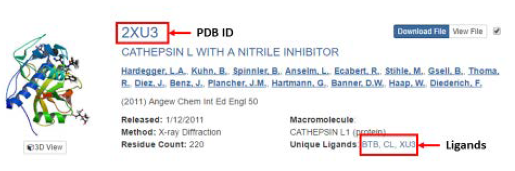
Additionally, have a look at the ligands that have been co-crystallized with the selected protein structure. These could be substrate, inhibitor, metal or buffer ion ligands.
The 3D interactions between the ligand and protein can be visualized by selecting the ‘Binding Pocket’ tab under any of the listed ligands. In this case, the inhibitor (XU3) is selected, and this directs us to a page showing the main interacting residues in the Cathepsin L binding pocket. Different display option can be selected based on preference.
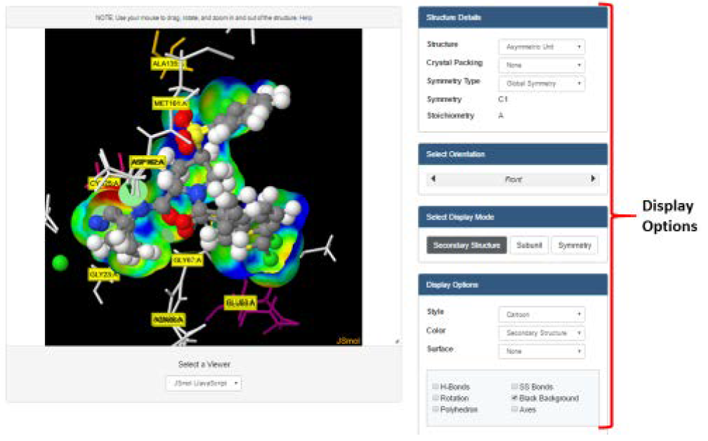
Although PDB provides this option to view protein-ligand interactions, this is limited to hydrogen bond interactions. By using PLIP, more and different protein-ligand interactions can be investigated, such as hydrogen and halogen bonds, hydrophobic contacts, pi-stacking and pi-cation interactions, and salt and water bridge interactions. PLIP also summarizes these interactions in an easy to read and comprehensible format, in addition to providing downloadable image and table files of the interactions, as well as Pymol session files of the detected interactions. Pymol is a non-web based visualization program that can be used additionally to view the interactions should one be familiar with it, although this is not necessary.
[2] Submit PDB structure to PLIP
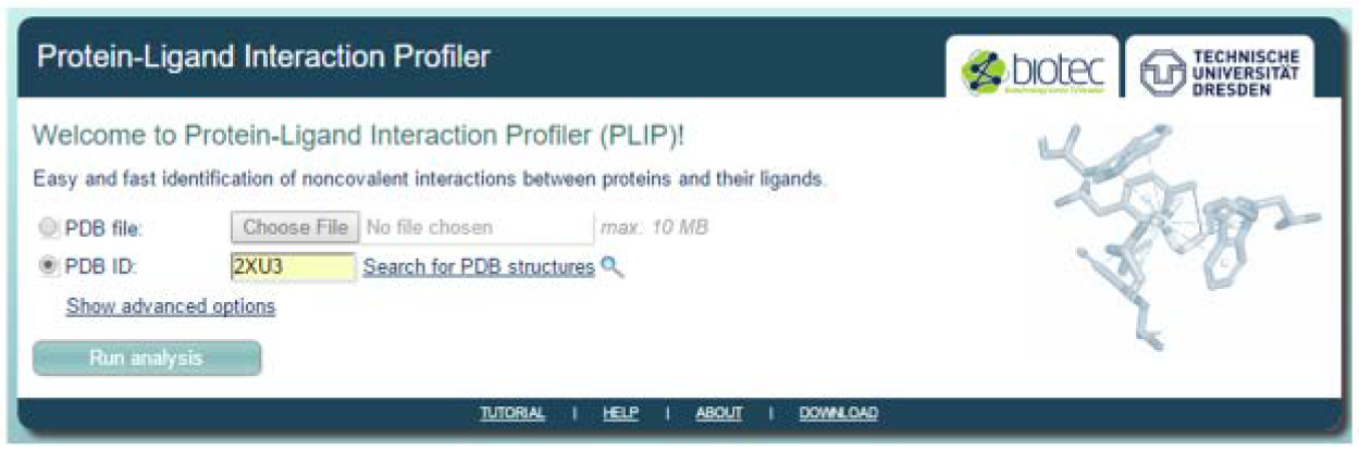
Go to the PLIP website: https://projects.biotec.tu-dresden.de/plip-web/plip/index and key in the PDB ID of your selected structure then click ‘Run analysis’. You can also choose to upload a structure that you have already download or a protein-ligand complex structure from the result of a docking experiment. You also have the option to enter a job name and your email address where the results can be sent to under ‘Show advanced options’.
[3] Analyze PLIP results
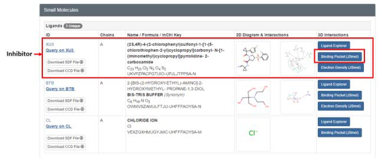
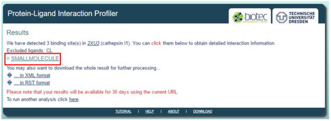
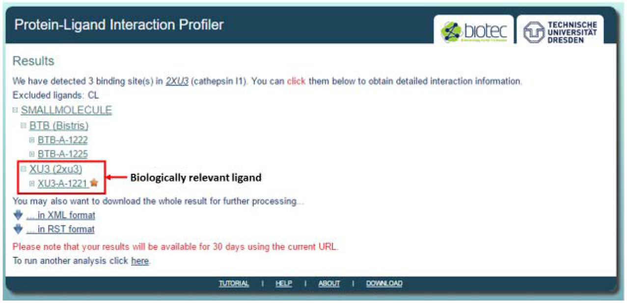
The results page will show the number of ligands detected as well as a summary of the interactions detected between each ligand at specified binding sites of the receptor protein. Click on the ‘Small Molecule’ tab.
The selected tab expands to show all the co-crystallized ligands, which can be further expanded. A star is next to the ligand is an indication of a biologically relevant ligand such as an inhibitor (XU3-A-1221), as opposed to the buffer ligands indicated in the example (BTB Bistris).
A summary of the profiled protein-ligand interactions is displayed upon further expansion of the biologically relevant ligand, in this case the inhibitor. This summary consist of a visual of the conformation of the ligand (orange) with respect to the receptor protein residues (blue) in the binding pocket, as well as the detected interactions as labeled according to the key on the right. The visual can be saved as a PNG image.
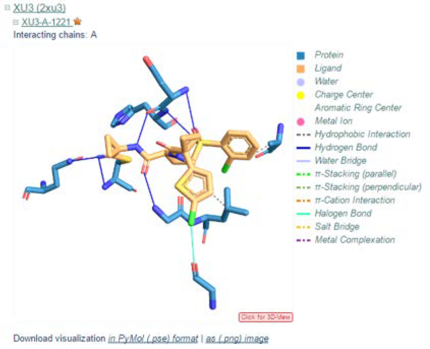
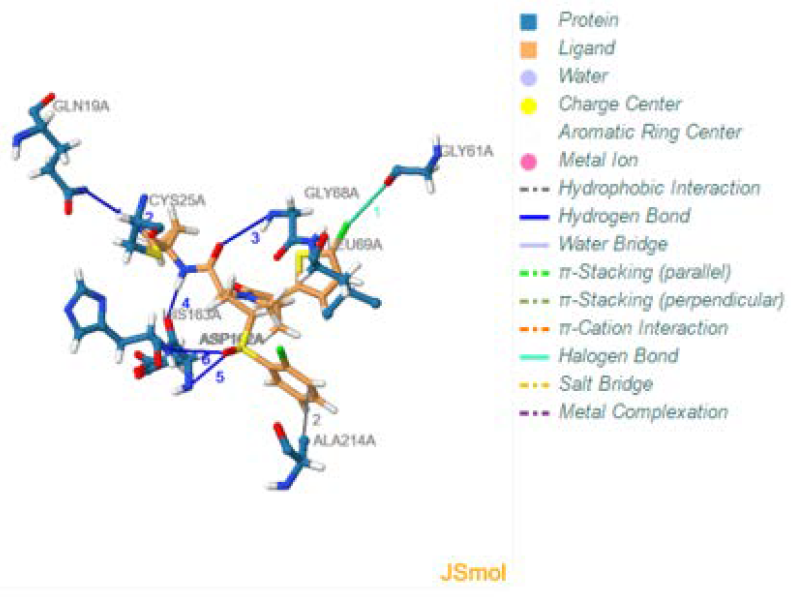
Furthermore, clicking on the ‘3D view’ option at the bottom of the visual will allow you to view the interactions in 3D where you can rotate the structure.
The bottom of the results page displays a tabulated summary of the specific interaction detected along with information corresponding to those interactions; such as a table displaying all the hydrogen bond interactions established, along with the specific interacting protein receptor residues, the donor and acceptor atoms, the bond angles and respective distances.
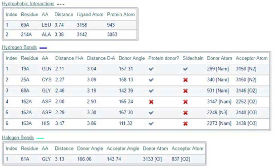
This tabulated information can also be downloaded to a suitable excel format and summarized according to preference. For instance, one can look at the hydrogen bonds across different inhibitors of various co-crystallized Cathepsin L structures. A tally or bar graph summary of the number of hydrogen bonds observed can be constructed to show the difference in the number of hydrogen bonds in each of the different ligand cases. This can be used in the inference of information about the binding affinities of ligands if the affinities are known, i.e. from experimental inhibitor studies or docking studies. Cathepsin L has a Cys25 residue that is involved and important for the catalytic mechanism of this enzyme. In this demonstration, this residue is detected to be involved in a hydrogen bonding with a nitrogen atom in the inhibitor (Hydrogen bonds table – Index 2). This amongst the other detected interactions indicates the effectiveness of the inhibitor against the protein receptor as the binding of the inhibitor directly prohibits the receptor from taking part in any catalytic interactions.
Protein motif analysis with MEME suite tools
AIMS:
To identify conserved motifs in protein sequences
OBJECTIVES:
- Choosing the right MEME suite tool for your problem
- Identify conserved motifs in protein sequences
- Identify conserved domains in protein sequences
EXPECTED OUTCOMES:
- To be able to use MEME suite tools in motif analysis
- To be able to identify conserved motifs and domains, and map them to sequence alignments
PRIOR PROTOCOL(S) REQUIRED FOR THIS PROTOCOL:
Retrieval of homolog sequences (NCBI and BLAST) and multiple sequence alignments
SUGGESTED NEXT STEP(S):
PDB and Visualization to map your motifs to structure
Background
Motifs are sub-sequences ~10–20 amino acids long within a larger set of related sequences that share common functionality and hence are conserved. They are the functional elements found in the domains -- functionally and structurally independent conserved regions within the sequence. This protocol is focused on motifs, but we will touch on the domains in passing to pique your interest to explore further.
The MEME Suite is a web server with a comprehensive collection of tools for nucleotide and protein motif analysis. It can be reached via http://meme-suite.org. See figure below for a list of the tools it hosts with a brief description of each.
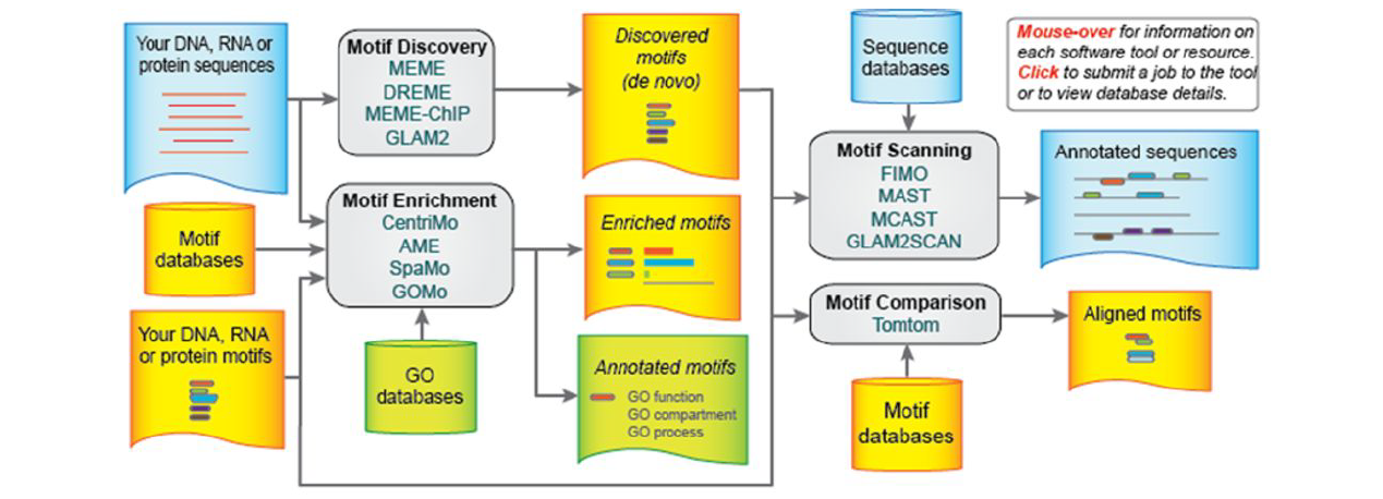

Timothy L. Bailey et al. Nucl. Acids Res. 2015;nar.gkv416
Step 1: Sequence retrieval
Retrieve the sequence of interest and its homologs. Avoid highly similar sequences to increase the chances of identifying essential motifs. See the “Retrieval of homolog sequences” section on how to do this.
Step 2: Define your problem
Why are you carrying out motif analysis? The results obtained during multiple sequence analysis (MSA) can guide you in answering this. Do you want to identify what the conserved regions observed in MSA are and do?
Step 3: Motif search with MEME
Search motifs using MEME, a tool that uses probabilistic techniques to identify un-gapped conserved motifs. Select MEME from the list of tools from the homepage.

Reasonable output can be obtained using the default optimized settings. However, you should be informed by prior information from MSA to determine the number of motifs to search for. The parameters of interest are annotated in the figure above, these are:
- Your uploaded FASTA-formatted sequences. MEME automatically check for errors and identifies the type of sequences entered
- Select the site distribution of your motifs. If you do not know how they are distributed, we recommend using ‘any number of repetitions’
- Increase the number of searched motifs to 10 or more
- Enter a Job description (recommended) and email address (optional)
Keep the advanced options as they are, since default options are optimized. The results are stored for a week and the recent jobs can be accessed via the sidebar until the computer is restarted. On submission, the job is queued and a summary is provided as shown below.

Step 4: MEME results
The motifs identified are returned represented as sequence LOGOS. Each position in the logo shows the amino acids that occur in that position while the height represents the level of conservation of the amino acid in that position.

The Sequence alignment provides an aligned list of regions in the sequences used to create the motif. Have a look at this, and try to locate them in your MSA.
In addition to the MEME results, the identified motifs are submitted to MAST -- a motif alignment and search tool -- with your original sequences as input to identify the locations of the motifs. We suggest you use its output as shown below to visually identify the locations of the motifs.

Compare this with your alignment results. Do you observe any similarity? Does it validate your alignment?
Step 5: Further analysis
The MEME Suite tools are interlinked, meaning that results from one tool can be directly submitted to another. For each motif, click on the arrow annotated “submit motif for further analysis. You will be presented with a dialog box like the one below.

From there, you can use the motif to search for its occurrence in other protein sequences e.g. UCSCC or Ensemble sequences. If you are curious, give them a try and see what you can glean.
Step 6: Gapped motifs
Some motifs may contain gaps, these will be identified by MEME as separate motifs. If you are interested in these gapped motifs, have a look at GLAM2 and GLAM2Scan. They are easy and direct to use.
Step 7: Where next?
At this stage, you should be able to choose the right tools for your sequences, identify motifs and search for their occurrence in other sequences. What, then, can you do from here?
Search for conserved domains in your sequences
- Conserved Domains Database (CDD) at http://www.ncbi.nlm.nih.gov/Structure/cdd/wrpsb.cgi
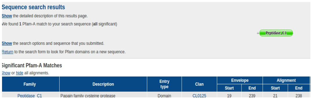
- Protein family database (Pfam) at http://pfam.xfam.org/

By searching conserved domains database with your sequence, you can figure out that these sequences are Cysteine proteases.
Explore other features in MEME-Suite
- For DNA sequences, the motifs are mostly transcription factor binding sites and promoter sites
- MEME-ChIP would be your go-to tool for motif identification, comparison and enrichment analysis
Be curious
Tinker with the settings, read through the MEME documentations and make use of the pop-up hints.
Physico-chemical properties of proteins
AIMS:
To analyze protein sequences for their physicochemical properties and deduce their characteristics.
OBJECTIVES:
- Be able to calculate pI, instability index, amino-acid composition, GRAVY (Grand average hydropathy), aliphatic index, estimated half-life, molecular-weight and total number of charged residues of protein sequences.
EXPECTED OUTCOMES:
- Understand protein functioning by deducing its attributes from calculated physicochemical properties evaluated by the ProtParam tool.
PRIOR PROTOCOL(S) REQUIRED FOR THIS PROTOCOL:
Retrieval of protein sequence in FASTA format from protein database. (See NCBI section)
SUGGESTED NEXT STEP(S):
Perform same calculation on other protein sequences in your dataset.
BACKGROUND:
Each of the 20 amino-acids in a protein structure contributes to its functioning, structural diversity and stability. Physico-chemical properties of these building blocks determine protein target specificity, its interaction with other proteins, co-factors and adjacent universe/environment. Such properties include molecular weight, bulkiness, Isoelectric point(pI), hydrophobicity, aromaticity, grand average of hydropathicity (GRAVY), instability index, aliphatic index and the overall amino-acid composition to name but a few.
Molecular weight provides information about the protein in terms of existence of monomers, dimers and conformational changes. It’s calculated by adding defined average isotopic masses of amino acids in the protein and the average isotopic mass of one water molecule. The values are presented in atomic mass units/Daltons. Molecular weight can be experimentally determined using SDS-PAGE.
Half-life prediction calculates the time taken for half of the protein to degrade after synthesis. This is partially influenced by the exposed N-terminal residue which may be removed during post-translational proteolytic processes. Half-life values correlate to protein function and cellular localization. E.g mitochondrial and endoplasmic reticulum proteins on average have longer half-lives.
Protonation or deprotonation of amino acids results in charged molecules. At isoelectric point (pI) the negatively and positively charged amino-acids are present in equal concentrations. pI values below 7.0 infer acidity. Acidity or basicity of a protein plays a major role in controlling its binding/target specificity and cellular penetration. Experimental distribution of charged molecules can be realized using electrophoresis.
Instability index estimates the stability of a protein in a test-tube. An index smaller than 40 is predicted as stable whereas an index greater than 40 means the protein may be unstable and thus have a shorter half-life.
Aliphatic amino-acids (alanine, valine, isoleucine and leucine) determine the aliphatic index. Aliphatic index describes the relative volume occupied by aliphatic side-chains. This index correlates to thermostability where the higher the value the more stable the protein is at higher temperatures.
GRAVY predicts the protein interaction with water molecules. It reflects their relative hydrophylicity and hydrophobicity. Lower values portray amicable interaction. Therefore lower GRAVY score (negative) would correlate to poor hydrophobic interactions thus the protein is characterized as hydrophilic. Positive scores show hydrophobicity. Most membrane-spanning proteins tend to have higher GRAVY values since they are composed of exposed hydrophobic regions that anchor the protein.
Amino-acid composition suggests its environmental and client protein/ligand interactions. Dominance of polar residues such as glutamine, threonine, tyrosine, serine, and histidine would indicate favorable interaction with water. Prevalence of charged amino-acids such as lysine, arginine, aspartate and glutamate would suggest a protein interaction with client proteins having oppositely charged residues thus target specificity.
STEP 1
You will require your input sequence you wish to analyze. For illustrative purposes the 5F02 crystal structure sequence (Uniprot ID: P07711) will be used as input. In your browser of choice you can access the ProtParam analysis tool from the Expasy website (http://web.expasy.org/protparam/).

STEP 2
To submit a sequence to the ProtParam analysis tool two options are available. The first option is to enter the accession number of the query sequence.
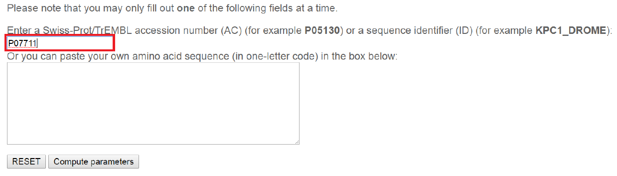
Alternatively the entire sequence can be copied from any text editor and paste it into the sequence field. When pasting the protein sequence ensure that the sequence name including the fasta symbol “>” is removed.
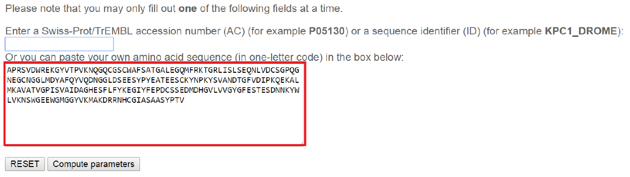
To execute the calculation click on the “Compute parameters” button.

STEP 3
The ProtParm tool will require end point of your sequence to be specified. These endpoints have to be above 5 residues long. The ProtParam tool will provide suggested endpoints which are based on sequence annotation information. Selecting one of these endpoints will perfom the analysis on only the selected region.

Alternatively the region of interest can be specified by specifying the start and end of the region in the fields below. This step can be skipped and the analysis will be performed on the entire protein sequence by clicking on the ‘SUBMIT” button.
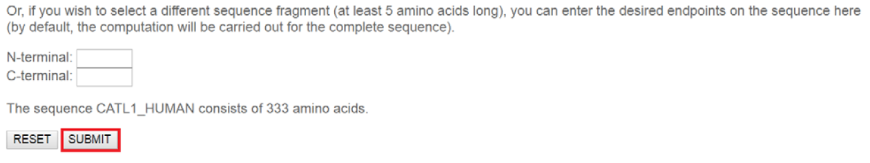
STEP 4
Once parameters have been computed a results page will be displayed. At the top of the results page will be displayed the user provided sequence which is your input sequence. All subsequent results are based on the displayed sequence.

In the results page physicochemical properties of the input sequence are summarized. The length of the query sequence is calculated based on the supplied amino acid sequence. The molecular weight of the protein is calculated in Daltons (Da) from the average isotopic masses of the amino acids. The theoretical pI derived from the Henderson-Hasselbalch equation is shown.

The occurrence frequency of all 20 standard amino acids are summarized in tabular format. The data may be exported to CSV file by clicking on the “CSV” button.

The number of positively and negatively charged residues in the query sequence is displayed. The total number of Aspartic acid (Asp) and Glutamic acid (Glu) denotes the negatively charged residues and the total number of Arginine (Arg) and Lysine (Lys) residues denotes the total number of positively charged residues.

A summary of the atomic composition of the input sequence can be found. The total number of atoms constituting each of the amino acids in the query sequence are summarized as a table. A molecular formula is shown based on atomic composition and the total number of atoms is summarized.

The extinction coefficient and absorbance of the query sequence is predicted to estimate how much light can be absorbed at a particular wavelength. Two predicted extinction coefficients are generated. The first extinction coefficient is calculated under the assumption that all Cysteine residues do not form salt bridges while the other coefficient assumes the opposite.
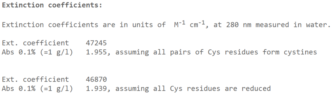
To infer the stability of the query protein sequence, the estimated half-life, Instability index and Aliphatic index are calculated. The half-life represents the predicted time it takes for the protein to decay when expressed in Human, yeast and E.coli. The instability index is a measure of how stable a protein is in a test tube. Proteins with Instability index below 40 are predicted to be stable while those above 40 are predicted to be unstable. The Aliphatic index is defined as the value of buried aliphatic residues (Alanine, Valine, Isoleucine, and Leucine). This measure is important for the thermostability of globular proteins. The GRAVY is indicative of how well the query sequence interacts with water. Proteins with a negative score are hydrophilic and those with a positive score are hydrophobic.

Protein interactions calculator (PIC)
AIMS:
Investigating the relative importance of various protein-protein interactions in the stability of the cysteine protease-chagasin complex
OBJECTIVES:
- To identify key inter-protein interactions using the Protein Interaction Calculator (PIC) web server
EXPECTED OUTCOMES:
- To be able to analyse inter protein interactions for a PDB of choice using the PIC web server
PRIOR PROTOCOL(S) REQUIRED FOR THIS PROTOCOL:
- Retrieval of 3D structures (See, PDB and visualization).
SUGGESTED NEXT STEP(S):
Map key residues to 3D structures (See PDB and visualization)
Investigate relative importance of interacting residues by mutation (See ROBETTA alanine scanning)
Introduction
In this protocol we will show how the Protein Interaction Calculator (PIC) and ROBETTA web servers can be used to investigate the relative importance of individual residues in specific protein-protein interactions between two proteins. As a case study we will demonstrate the necessary methodology by analyzing the key interactions between a cysteine protease in complex with chagasin, a potential cysteine protease inhibitor. In our analysis we will first identify the residues in cysteine protease that contribute to protein-protein interactions with chagasin. Following this analysis, the relative importance of these residues in maintaining the stability of the cysteine protease-chagasin complex will be investigated and validated using in silico mutations in a process call alanine scanning (see ROBETTA alanine scanning protocol).
Protein interaction calculator methodology
The Protein Interactions Calculator (PIC) is a web server that recognizes various kinds of interactions within a protein or between proteins in a complex, based on empirical and semi-empirical rules. All the server requires is a file of the molecular structure(s) in the Protein Data Bank (PDB) format.
- Retrieve the cysteine-protease-chagasin complex from the protein data bank (PDB ID: 2OUL)
- View the complex in a molecular graphics viewer such (see PDB and visualization protocol), and familiarize yourself with the orientation of each molecule
- Use the PIC webserver to obtain information regarding the protein-protein interactions between the cysteine protease (chain A) and chagasin (chain B)
- The PIC webserver can be accessed using the following link http://pic.mbu.iisc.ernet.in/
- On the home page follow the link indicated below to submit a new job to the PIC webserver
- PIC has several protein interaction calculators; intra-protein and protein-protein interactions, solvent accessibility based calculations, and depth calculations. In this case study we are interested in looking at interactions between protein molecules and thus protein-protein interactions will be used.
- Scroll down the submit job page until you find the subsection titled Protein-Protein interactions (see below figure)
- Here you will be required to upload your molecular structure in PDB file format. Upload 2OUL.pdb
- PIC allows the user to choose which interaction types should be calculated (hydrophobic interactions, disulphide bridges, hydrogen bonds, ionic interactions, aromatic interactions, and cation-Pi interactions), because we are unsure what interactions are important between our protease and chagasin we will select all interaction types
- Note that the user can also set their desired cut-off values in Å for bond lengths, we will leave all of these to default by leaving them blank
- By entering in your email address the PIC server will conveniently email you your results, allowing you to view them again at a later date.
- Once all required and optional parameters are filled in, click the “Submit Query” button to send your job to the PIC webserver
- DO NOT close your web browser or tab if you did not enter in your email address as the server will redirect you to a results page once the calculations are complete
- The waiting period for your results will depend on the total size of your molecular structure. On average this shouldn’t take more than 4 min
- If you entered your email address into the job submission, a copy of your results should be available in your inbox shortly after the calculations are complete
- If you did no opt for the email option, your web browser will redirect you away from the submissions page to your results page
- The results for all the selected interaction types appear together on this results page, listed one after the other in the following order; hydrophobic interactions, disulphide bridges, hydrogen bonds, ionic interactions, aromatic interactions, and cation-Pi interactions. Depending on which interactions were originally chosen.
- You will notice for our case study that there is data listed for; hydrophobic interactions, hydrogen bond, ionic interactions and aromatic-aromatic interactions. PIC will print out a message in the results page informing the user if no interactions of a specified type are present.
- For those interactions for which data was found, PIC reports several columns of data depending on the interaction type. For this case study PIC reports a total of 14 hydrophobic interactions within the default 5Å cut-off between the protease (chain A) and chagasin (chain B) in our complex. For each interaction PIC also reports the name and position for each residue involved as well as their respective chains (note that this information is based strictly on the PDB data, not protein sequence).
- Looking at the first entry, PIC reports a hydrophobic interaction between TRP26 in chain A (blue box) and LEU65 in chain B (red box). Where chain A represents the protease, and chain B the chagasin.
- At a glance it is clear that some residues in the protease (chain A) have multiple hydrophobic interactions with several different residues in the chagasin (chain B) i.e. residues 67, 140 and 141
- By removing the duplicates in this list we can conclude that 11 residues in the protease are involved in hydrophobic interactions with chagasin residues. Specifically; TRP26, TYR61, LEU67, ILE68, VAL135, ALA140, PHE141, LEU155, ALA158, TRP189 and TRP193
- The remaining data for the other interaction types can be interpreted in a similar manner, however care should be taken when looking at interactions such as hydrogen bonding where it is important to consider bond length and bond angle which is conveniently supplied by PIC. The interpretation of these data is up to the user alone and must therefore be done with care.
- The data for hydrogen bonds is thus slightly different to the other interaction types. PIC separates the data into donor residues (blue box), and acceptor residues (red box), again reporting the residues name, position and chain, but also including the donor or acceptor atom, i.e. N or O. Furthermore PIC reports the distance between the donor and acceptor atoms as well as the distance between the hydrogen and acceptor atom. Furthermore all bond angles are reported.
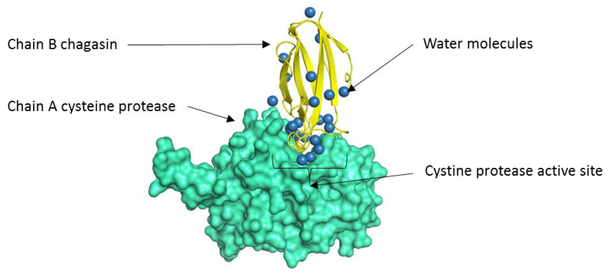
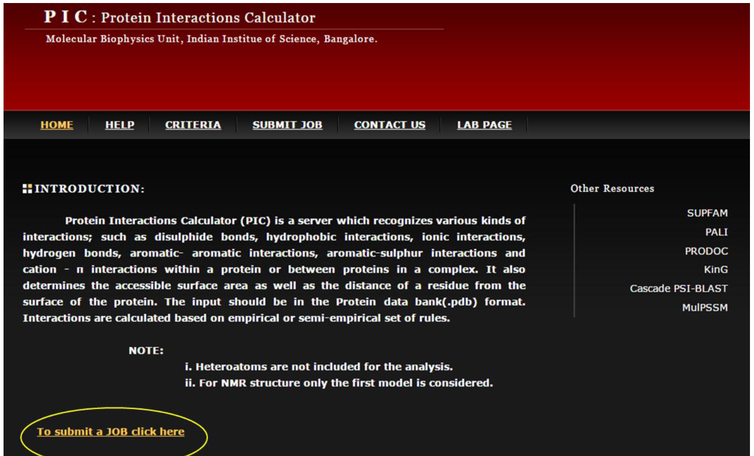
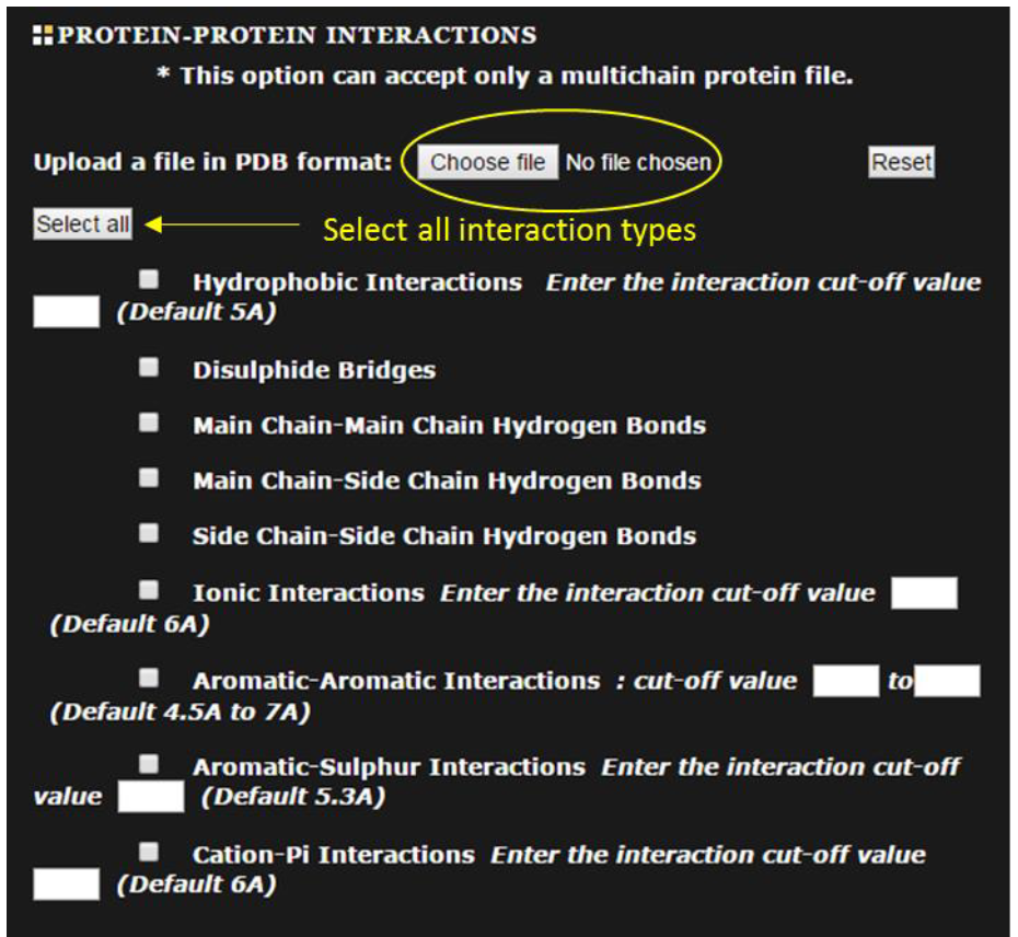

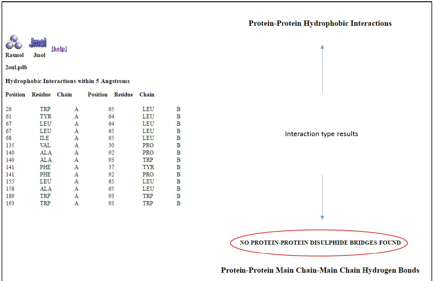
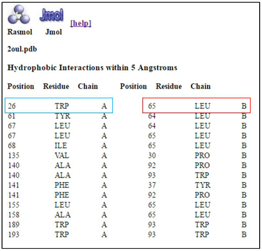
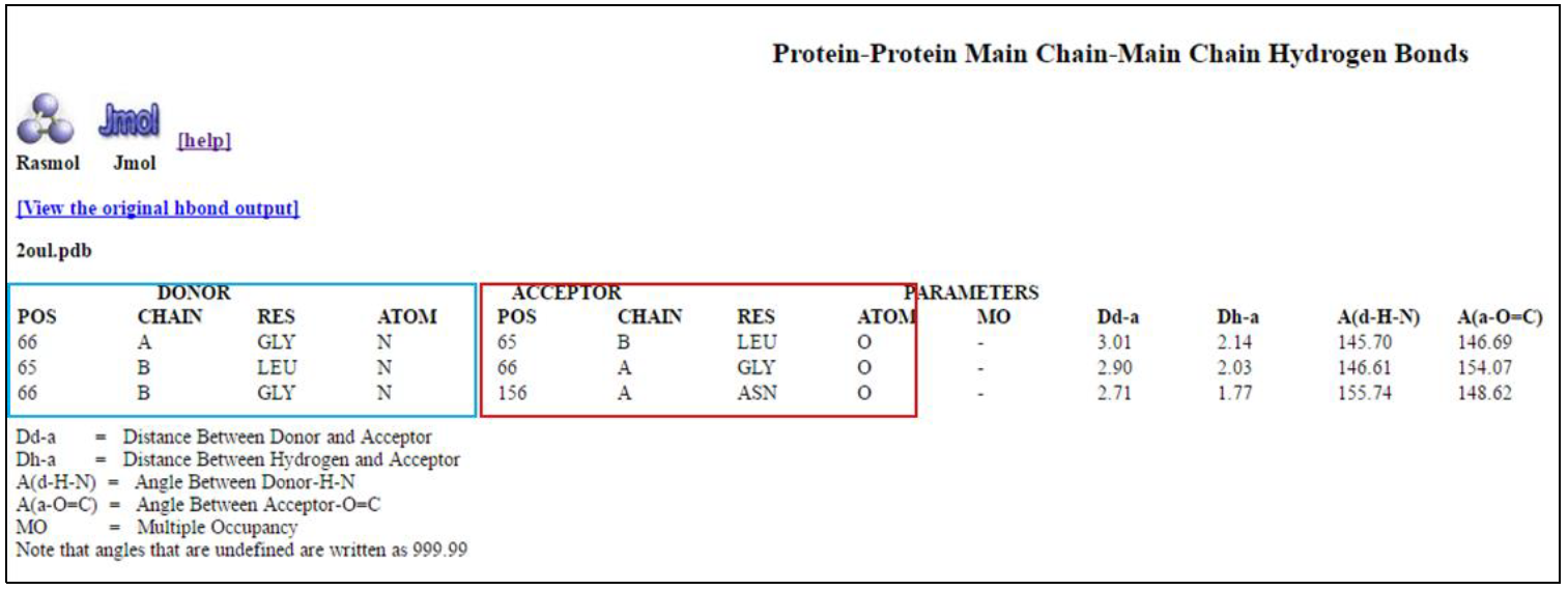
Results
By analyzing the PIC data and removing all interaction type duplicates, it is possible to compile a list of residues in the cysteine protease that play a role in protein-protein interactions with chagasin (see table below) (note that residue numbering is based strictly on the PDB data, not protein sequence).
| Interaction type | Residues |
|---|---|
| Hydrophobic | 26,61,67,68,135,140,141,155,158,189,193 |
| Hydrogen bond | 18, 19, 66, 154, 156, 157, 189 |
| Ionic | 18, 137, 153 |
| Aromatic | 141, 189, 193 |
This data can be represented visually using protein visualization software (see PDB and visualization protocol).
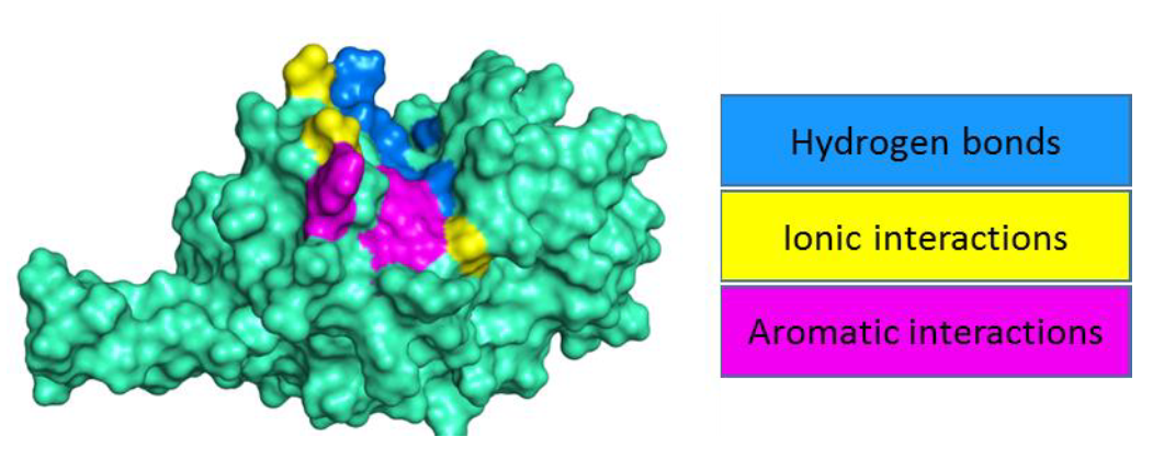
ROBETTA alanine scanning
AIMS:
Investigating the relative importance of various protein-protein interactions in the stability of the cysteine protease-chagasin complex
OBJECTIVES:
- Given a known set of cysteine protease residues predicted to interact with chagasin, use the ROBETTA alanine scanning protocol to investigate the change in stability of the complex upon mutation of these residues to alanine.
EXPECTED OUTCOMES:
- To be able to perform computational alanine scanning for a specific set of interface residues within a protein-protein complex.
- To understand the use of the ROBETTA web server
PRIOR PROTOCOL(S) REQUIRED FOR THIS PROTOCOL:
- Retrieval of 3D structures (See, PDB section)
- Protein interactions calculator (PIC)
SUGGESTED NEXT STEP(S):
Map key residues to 3D protein structures (See PDB and visualization)
Introduction
In this protocol we will analyse the relative importance key inter-protein interacting residues (see Protein Interaction Calculator protocol) in the cysteine protease-chagasin complex in maintaining the stability of this protein-protein, by mutating each residue to alanine and observing the relative effect.
ROBETTA Alanine Scanning
Introduction
The ROBETTA webservers offers a range of tools for the modeling and analysis of protein structures. Included in the package is a computational alanine scanning protocol for the analysis of protein-protein interfaces. An interface residue is defined, by ROBETTA, to contain one or more atoms within a sphere with 4Å radius of an atom belonging to the partner subunit. It must also be noted that ROBETTA excludes glycine and proline residues from the analysis. Computational alanine scanning uses a free energy function to calculate the effects of individual alanine mutations on the binding free energy of a protein-protein complex. To interpret these effects, we must first understanding the concept of binding free energy:
Free energy of a system:
DEFINITION: The free energy of a system is a thermodynamic potential that measures the capacity of a system to do work. Alternatively it is the potential energy of the system. In this case, the binding free energy is the free energy to create potential complexes.
Binding energy:
DEFINITION: The binding energy is the energy required hold the complex together as a stable entity. Alternatively it is the energy required to separate a bound state into its separate units.
INTERPRETATION: A bound complex will contain less potential energy than the sum of its separated parts. This is because when a complex is formed, there is a decrease is the free energy (or potential energy) of the complex because energy is now required to stabilise the complex. This stabilising energy in the binding energy. However when the complex is destabilised, or separated into its individual parts, this binding energy is released and the potential energy (free energy) or the complex increases.
Interpreting ROBETTA results:
ROBETTA calculates the change in binding free energy of a complex upon a mutation of a single residue to alanine. The effects can be interpreted as follows:
1) Increase in binding free greater than 1 kcal/mol is associated with destabilsation
2) Decrease in binding free energy less than -0.8 kcal/mol is associated with stabilisation of the complex.
3) Neutral mutations cause a change in binding free energy from -0.8-1 kcal/mol.
Aim of this investigation
Currently, we have used PIC to determine which cysteine protease interface residues are important for the interactions between cysteine protease and chagasin, a potential cysteine protease inhibitor (PDB ID: 2OUL). In total we identified 19 interacting residues in the cysteine protease protein:
| Interaction type | Residues as labeled in PDB file |
|---|---|
| Hydrophobic | 26,61,67,68,135,140,141,155,158,189,193 |
| Hydrogen bond | 18, 19, 66, 154, 156, 157, 189 |
| Ionic | 18, 137, 153 |
| Aromatic | 141, 189, 193 |
We will now take this investigation further, and use ROBETTA computational alanine scanning to systematically mutate each of these residues and determine the respective effects on complex stability. This will allow us to identify key interacting residues responsible for the stability of the complex.
Methodology
- Registration: The ROBETTA webserver requires all users to register. You can register at the following link: http://robetta.bakerlab.org/register.jsp
- Once registered, you can start to use the ROBETTA Interface Alanine Scanning. You can submit your job at the following link: http://robetta.bakerlab.org/alascansubmit.jsp . An example of the submit form is shown below:
- Input Requirements:
- User-name or email: user-name or email that you registered
- Job name: a name of your choice
- Complex: click browse and upload the saved PDB file: 2OUL.pdb
- Partner Definitions:
- Upload mutations list: this is a list of the specific residues that you would like to mutate to alanine. In our case it will include a list of the 19 cysteine protease (falcipain 2) residues that we previously identified using PIC.
- Column 1: The residue number as in the PDB complex
- Column 2: The chain ID as in the PDB complex (case sensitive). In our investigation this will always be Chain A, as we are only mutating the 19 Falcipain 2 residues.
- Column 3: Experimental delta delta G values. As we do not know these values we will define all values as 0.00
- Submitting the job: once all input requirements have been correctly filled in, the job can be submitted to the server. Simply click the “Submit” button. An example of the correct form for submission is given below.
Here you will create a user-name and register your email address. After submitting a run, a link to the results will be sent to this email.
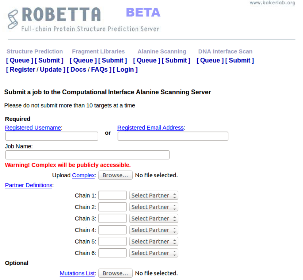
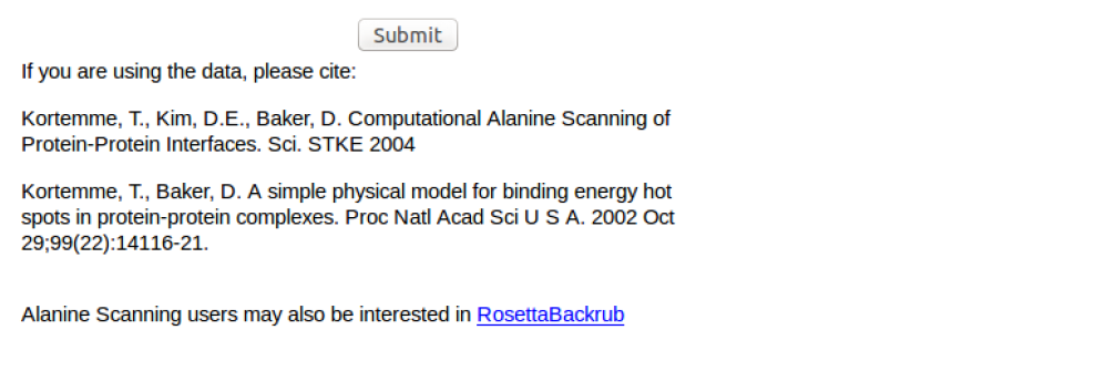
The PDB complex consists of two chains:
Chain A: Cysteine Protease Falcipain 2
Chain B: Chagasin
We are interested in the stability of the interface between these two proteins. Therefore these two chains will be defined as the interacting partners as follows:
- Chain A will be Partner 1
- Chain B will be Partner 2
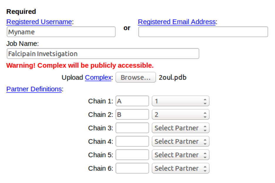
Note that the chain labels must correspond to the labels in the PDB file. If you are using a different protein and the chains are labeled as Chain 1 and Chain 2, the Partner Definition will be:
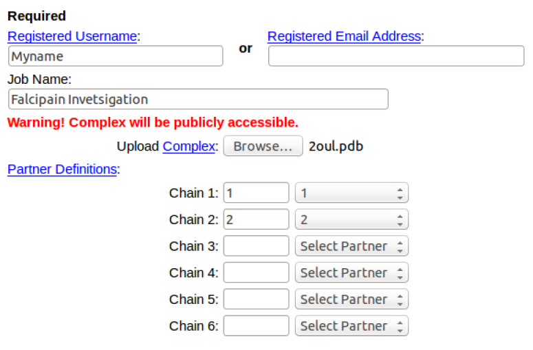
Note: The mutations list is an optional input. If it is excluded, ROBETTA will mutate all interface residues.
Preparation of the mutations list:
- The list must be prepared as a txt file.
- It must contain 3 columns, each column separated by a single space
- Note: If there are any format errors then all interface mutations will be considered.
Example of the Mutations.txt used in this study.
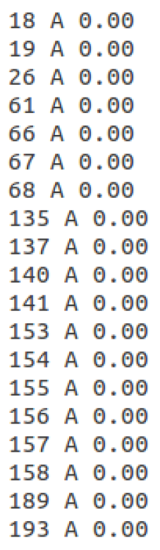
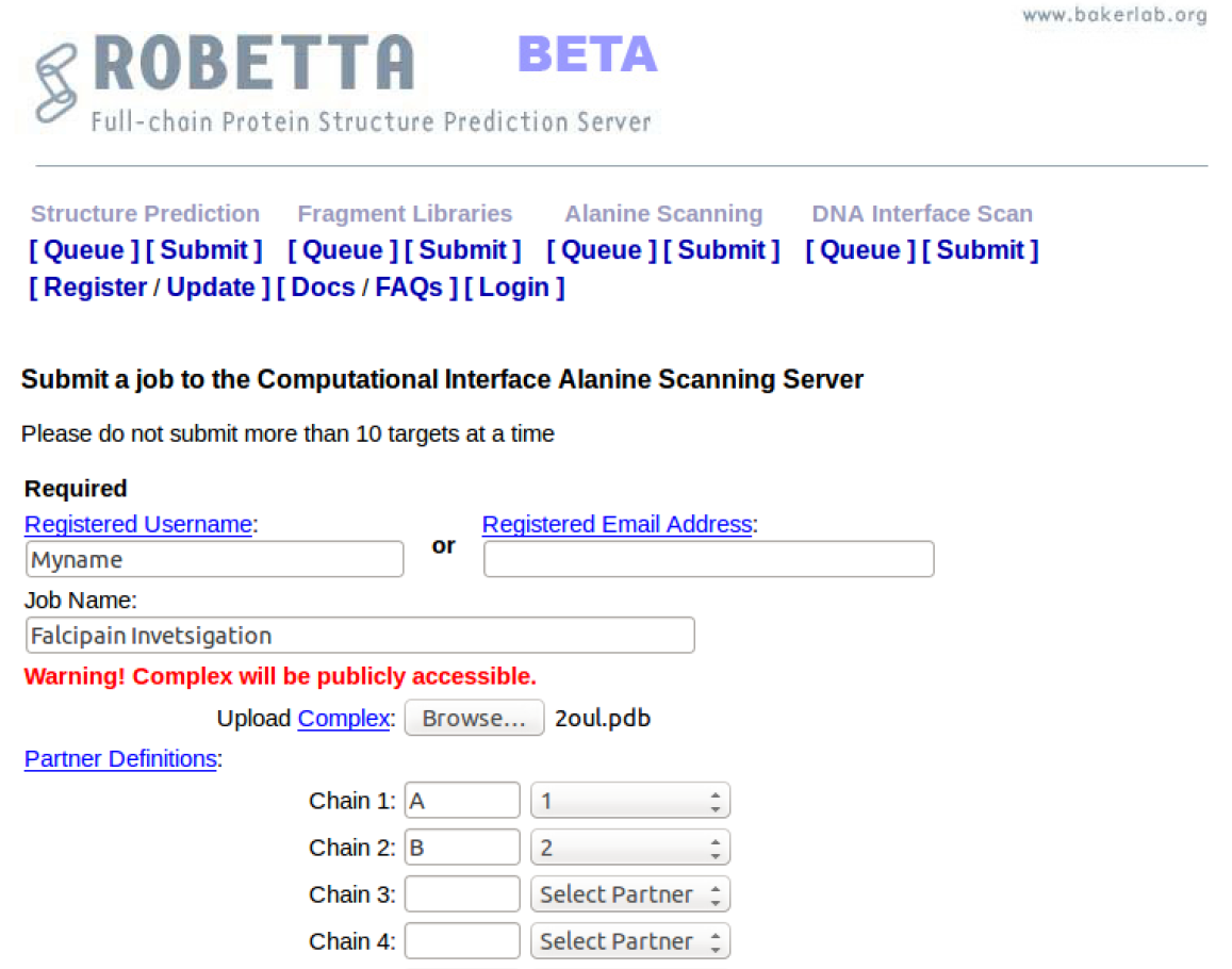
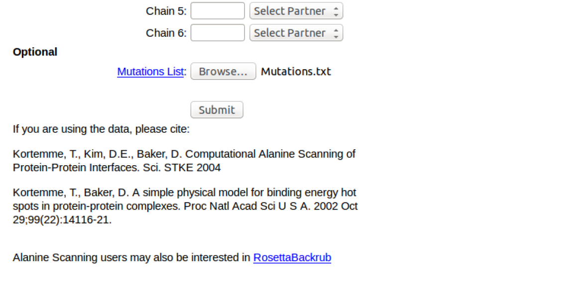
Retrieving Results
The results may be retrieved in two ways:
- From the queue.
- Through a link in your email
To access your results from the queue, click the link on the ROBETTA home page to the alanine scanning queue:
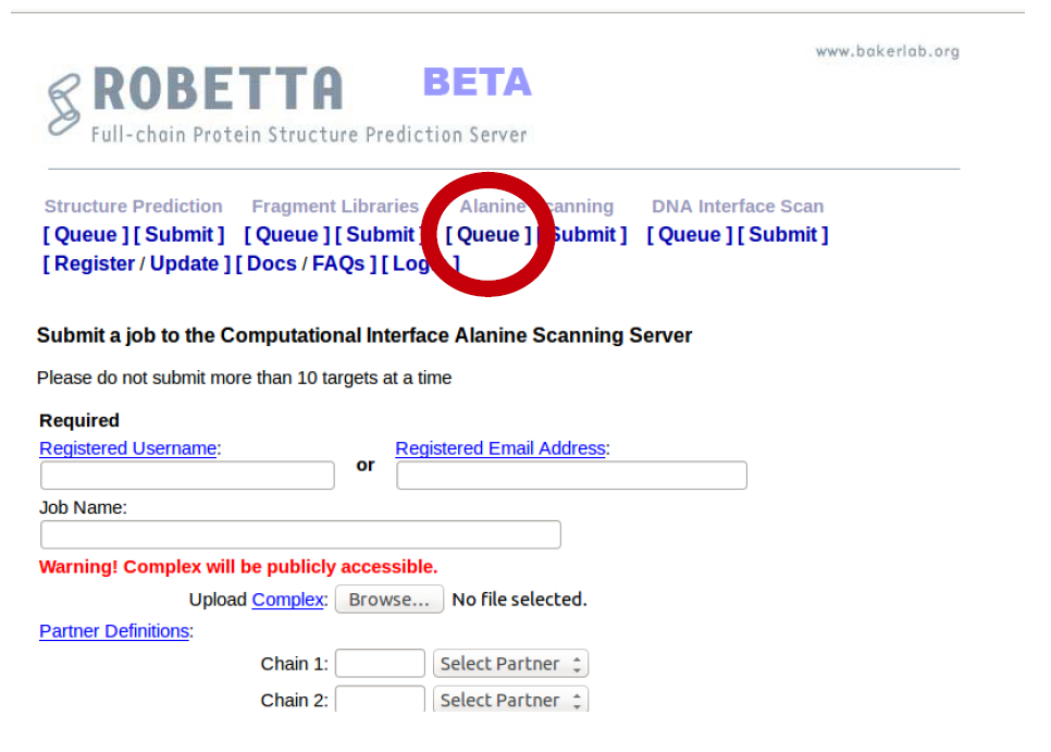
If your job is complete you will be able to access your results by clicking on the link “Complete”:
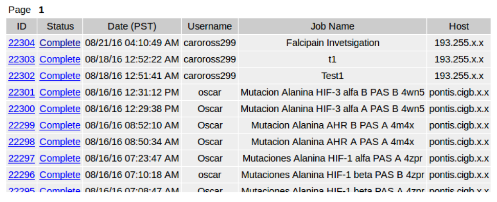
The output will include a series of files, including a text file 2oul.alascan.results. This is a text file which will tell us the change in binding free energy, per mutation. The results given for this case study are shown below:
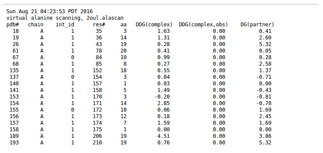
This text file can also be retrieved from a link which will be sent to your registered email address.
Analyzing the Results
The file 2oul.alacan.results contains the following columns:
- pdb#: the number of the residue as given in the PDB file 2oul.pdb
- chain: the chain in which the mutated reside is located
- int_id: measure of whether a residue side chain atom is within 4 Å of an atom on the other partner. 1) Atom is within 4 Å of an atom on the other partner. 0) Not contacting directly, but buried upon binding.
- res#: Continuous residue numbering of all partners- determined by ROBETTA.
- aa: amino acid type according to one-residue nomenclature in alphabetical order
- DDG (complex): change in binding free energy of the full Falcipain-Chagasin complexes
- DDG (complex, obs): observed changes in binding free energy upon alanine mutation (user input in mutation list, otherwise set to zero). In our case it will be zero as we did not define the experimental data.
- DG (partner): predicted change in protein stability of the individual partner. In our case this refers to Chain A: Falcipain 2.
Our analysis focuses on columns 6 and 8. From analyzing this data we can determine which mutations destabilised the Falcipain- Chagasin complex and which mutations destabilised the Falcipain protein. REMEMBER: a destabilising mutations results in a predicted increase in binding free energy greater than 1 kcal/mol.
Results
- In this case study we identify 6 Falcipain 2 residues, predicted to interact with Chagasin, that destabilised the Falcipain- Chagasin interface when mutated to alanine, 3 of which also destabilised the individual Falcipain protein.
- We also identify an additional 6 residues that only destabalised the individual Falcipain protein.
These results are shown in the table below.
| Residue | Interaction determine by PIC | DDG (complex) | DG (partner) |
|---|---|---|---|
| D18 | Hydrogen Bonding | 1.63 | 0.41 |
| Q19 | Hydrogen Bonding | 1.31 | 2.60 |
| W26 | Hydrophobic | 0.28 | 5.32 |
| I68 | Hydrophobic | 0.27 | 2.58 |
| V135 | Hydrophobic | 0.55 | 1.37 |
| F141 | Aromatic, Hydrophobic | 1.49 | -0.43 |
| Q154 | Hydrogen Bonding | 2.85 | -0.78 |
| L155 | Hydrophobic | 0.06 | 1.69 |
| N156 | Hydrogen Bonding | 0.18 | 2.45 |
| H157 | Hydrogen Bonding | 1.59 | 1.69 |
| W189 | Aromatic, Hydrophobic | 4.51 | 3.86 |
| W193 | Aromatic, Hydrophobic | 0.76 | 5.32 |
Single Nucleotide olymorphism (SNP) effect prediction
AIMS:
Use in silico web-based tools such as PredictSNP to predict which SNPs in the p53 tumor suppressor gene are likely to be associated with cancer
OBJECTIVES:
- Use PredictSNP to predict the effects of selected SNPs in the p53 tumor suppressor protein
- Identify SNPs in the p53 gene that are likely to be associated with cancer
EXPECTED OUTCOMES:
- A table showing potentially deleterious or benign SNPs in the p53 tumor suppressor gene
PRIOR PROTOCOL(S) REQUIRED FOR THIS PROTOCOL:
Retrieval of data from NBCI and Uniprot
SUGGESTED NEXT STEP(S):
Protein modeling and Protein-ligand interaction analysis
Introduction
Genetic variations play a crucial role in human phenotypic traits and ultimately disease. Single nucleotide polymorphisms (SNPs) are the most frequent type of genetic variation in humans. SNPs account for over 85% of mutations associated with disease [1]. The effects range from truncation of proteins by introducing stop codons in extreme cases resulting in complete loss of protein function. In other instances, the effects are subtler, for example affecting protein folding and stability ultimately impairing their ability to catalyze reactions or bind ligands.
Perhaps one of the best studied examples is Sickle cell anemia [2, 3]. In the illustration you can see normal red blood cells (RBCs) besides a sickled RBCs. (Illustration from Anatomy & Physiology, Connexions Web site: http://cnx.org/content/col11496/1.6/, Jun 19, 2013). This is the result of a rs344 SNP in the hemoglobin gene. Hemoglobin is the protein responsible for oxygen transport in the RBCs. The mutation from the A ancestral allele to the T allele results in a codon change from GAG to GTG leading to a translation change from Glutamine (E) to Valine (V). The mutation results in a disease which is severe, causing pain, and anemia. People who carry only one copy of the mutant gene are carriers and have the potential to pass on the disease to their offspring.
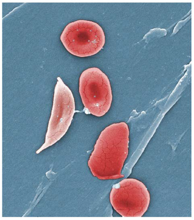
In silico prediction of the effects of SNPs on the translated protein structure and function is a largely under-explored area. We know that SNPs can result in diseases, but we also know that they can influence individual responses to chemotherapeutics which is fairly important in the era of personalized medicine [4, 5]. SNP effect prediction programs typically classify SNPs as either deleterious or of no consequence/neutral/benign. Some tools use conservation based measures [6]. Others use a combination of both conservation based methods as well as structural features in conjunction with machine-learning approaches such as support-vector machines or neural networks [7–10].
In this protocol the freely available web-server PredictSNP [11] (http://loschmidt.chemi.muni.cz/predictsnp1/) will be used.
EXERCISE:
p53 tumor suppressor protein
As the name suggests this protein is involved in protecting your body from cancer. Impairment of this protein results in a loss of the body’s normal defense that protects against uncontrolled cell growth. p53 mutations contribute to almost half of the cases of human cancer [12].
In this study we will explore the effects of missense SNPs (SNPs that result in a codon change that results in an incorrect amino acid at one point in the protein sequence) on p53. In instances where p53 function is impaired, the protein is unable to stop uncontrolled multiplication of potentially cancerous cells and thus unable to prevent formation of tumors.
p53 protein sequence (UniProt ID: P04637-1)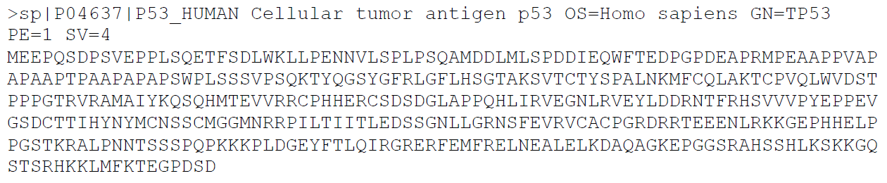
Missense SNPs and amino acid substitutions
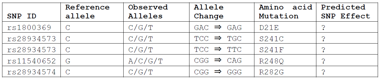
STEP ONE: Submission of query
- Go to the predict SNP website and select the ‘Consensus classifier for prediction of effect of amino acid substitutions’
- Paste the UniProt sequence into the search window and click the load button
- Under ‘MUTATIONS’ tab using your cursor select which residues to mutate (refer to Table 1) and indicate which amino residues to mutate to in the ‘select mutations’ option. The final input should look like the screen-shot below.
- Once you have finished selecting the mutations under the “TOOLS FOR EVALUATION” tab select which SNP prediction tool (or tools) you would like to use. We recommend you use at least seven for better comparison of the prediction results. For each tool a predicted duration time is given along with its expected accuracy. Enter your email address and job title (optional). The duration of your run will depend on how many jobs are in the PredictSNP queue. Click on ‘Evaluate’ to begin the job.
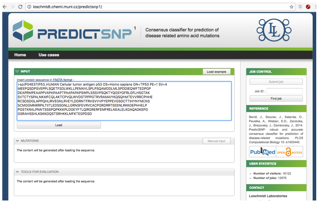
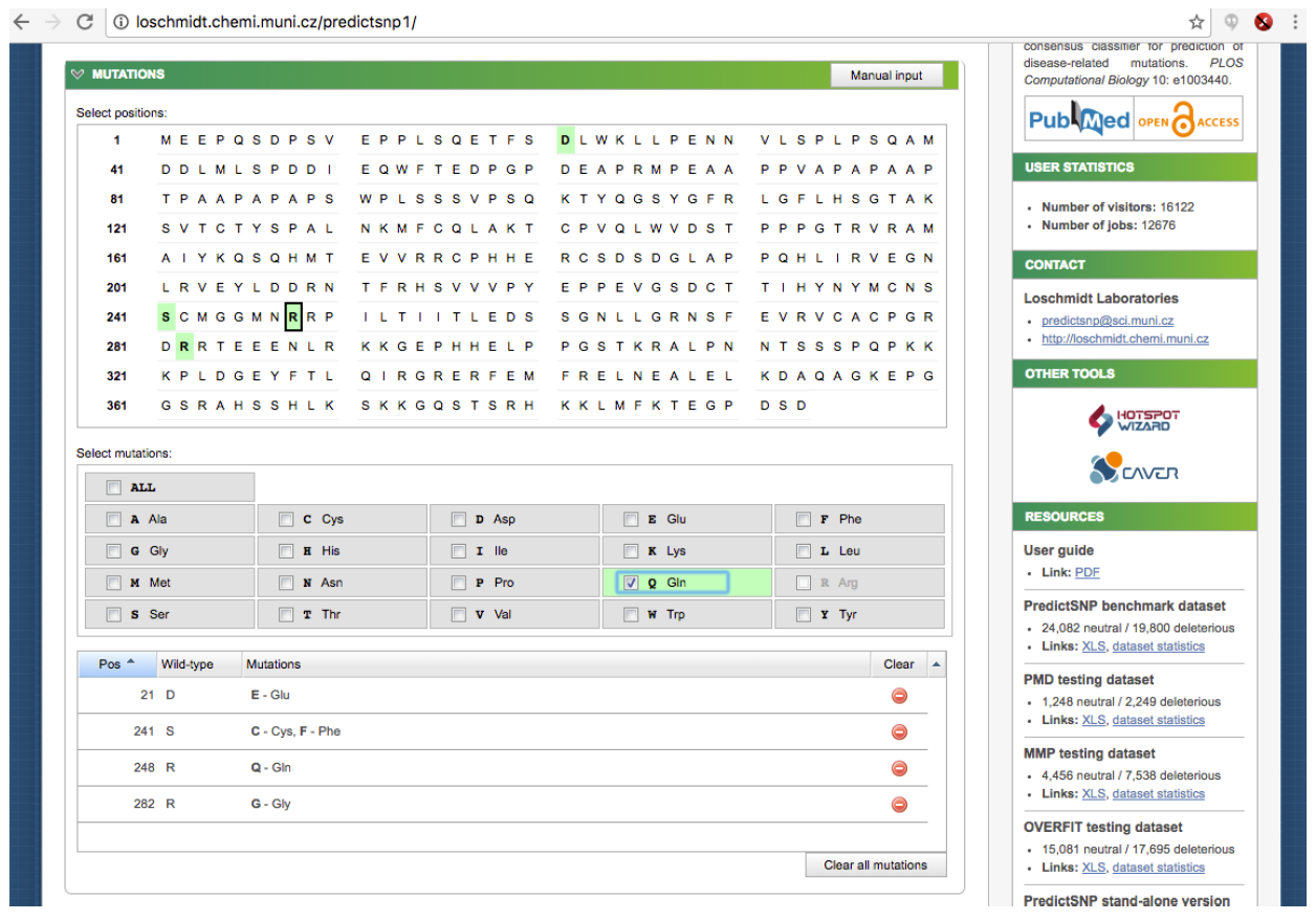
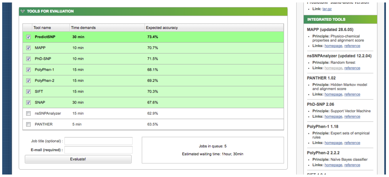
STEP TWO: Evaluation of results
Please note that what these in silico tools provide are predictions. To conclude whether any of these SNPs actually result in cancer requires further analysis/analyses. For example: protein modeling or genetic association studies.
- The results when ready appear as shown in the screen-shot below giving a consensus value for each of the SNPs in the PredictSNP column. You can hover your cursor over the value to get the confidence of the prediction for each value. If you click the ‘Download’ tab you can download the results as a comma separated value file (‘.csv’) that you can open in excel.
- PredictSNP where possible provides annotation information on the SNPs which can be useful. Click on ‘Expand all annotations’ to see the available annotation information.
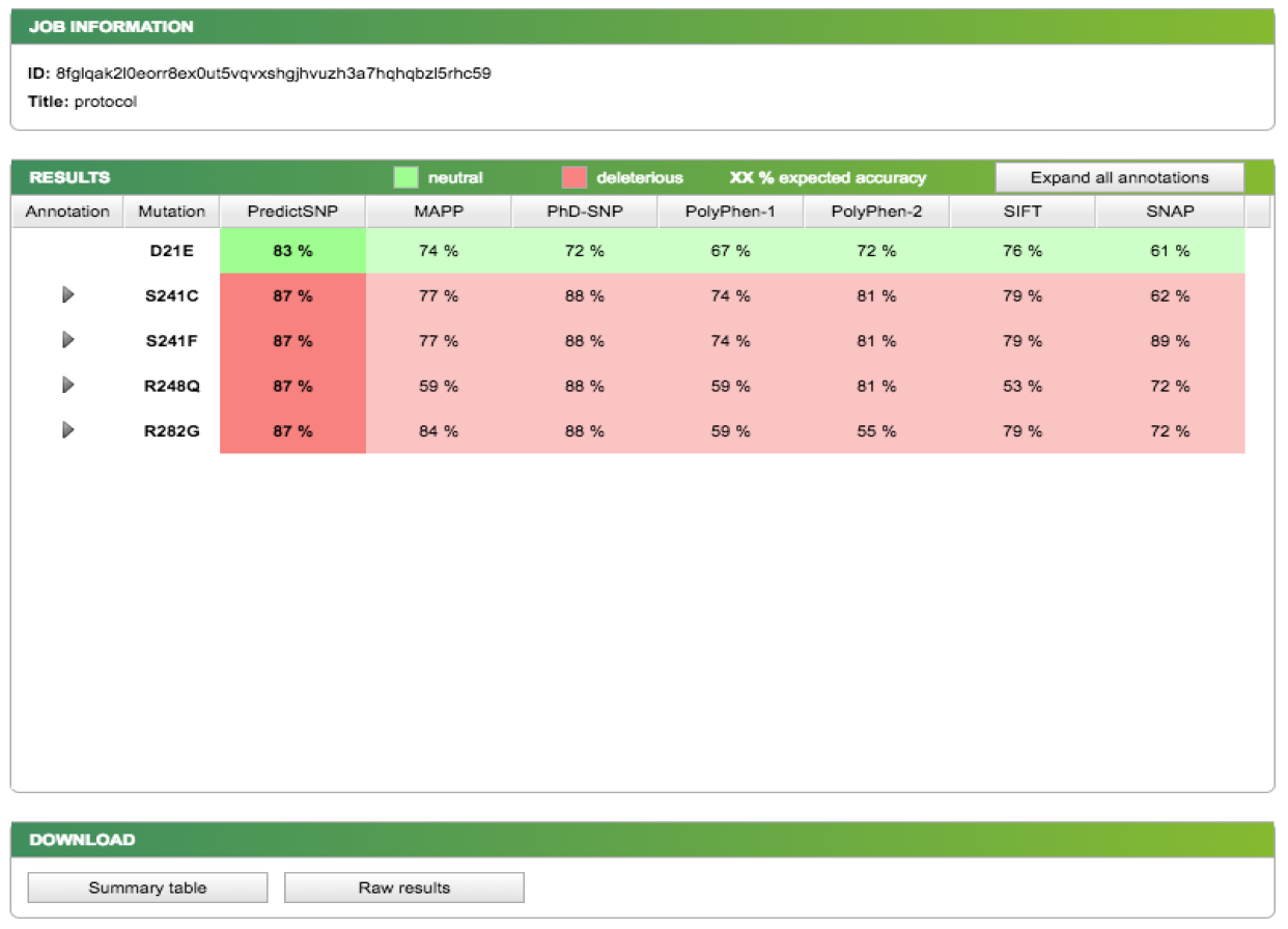
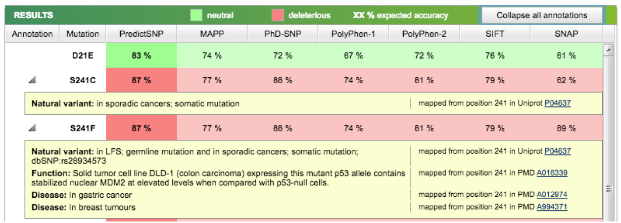
Complete the predicted SNP effect column in exercise Table 1. Do the results tally with the available literature on the SNPs?
REFERENCES:
1. McKenna A, Hanna M, Banks E, Sivachenko A, Cibulskis K, Kernytsky A, Garimella K, Altshuler D, Gabriel S, Daly M, DePristo MA: The Genome Analysis Toolkit: a MapReduce framework for analyzing next-generation DNA sequencing data. Genome Res 2010, 20:1297–303.
2. Steinberg MH, Sebastiani P: Genetic modifiers of sickle cell disease. American Journal of Hematology 2012:795–803.
3. Rees DC, Williams TN, Gladwin MT: Sickle-cell disease. Lancet 2010, 376:2018–31.
4. Fernald GH, Capriotti E, Daneshjou R, Karczewski KJ, Altman RB: Bioinformatics challenges for personalized medicine. Bioinformatics 2011, 27:1741–1748.
5. Giacomini KM, Brett CM, Altman RB, Benowitz NL, Dolan ME, Flockhart D a, Johnson J a, Hayes DF, Klein T, Krauss RM, Kroetz DL, McLeod HL, Nguyen a T, Ratain MJ, Relling M V, Reus V, Roden DM, Schaefer C a, Shuldiner a R, Skaar T, Tantisira K, Tyndale RF, Wang L, Weinshilboum RM, Weiss ST, Zineh I: The pharmacogenetics research network: from SNP discovery to clinical drug response. Clin Pharmacol Ther 2007, 81:328–345.
6. Kumar P, Henikoff S, Ng PC: Predicting the effects of coding non-synonymous variants on protein function using the SIFT algorithm. Nat Protoc 2009, 4:1073–1081.
7. Adzhubei I, Jordan DM, Sunyaev SR: Predicting Functional Effect of Human Missense Mutations Using PolyPhen-2. In Current Protocols in Human Genetics. Volume Chapter 7; 2013(January):7.20.1-7.20.41.
8. Sunyaev S, Ramensky V, Bork P: Towards a structural basis of human non-synonymous single nucleotide polymorphisms. Trends Genet 2000, 16:15–17.
9. Bromberg Y, Rost B: SNAP: Predict effect of non-synonymous polymorphisms on function. Nucleic Acids Res 2007, 35:3823–3835.
10. Venselaar H, Te Beek T a H, Kuipers RKP, Hekkelman ML, Vriend G: Protein structure analysis of mutations causing inheritable diseases. An e-Science approach with life scientist friendly interfaces. BMC Bioinformatics 2010, 11:548.
11. Bendl J, Stourac J, Salanda O, Pavelka A, Wieben ED, Zendulka J, Brezovsky J, Damborsky J: PredictSNP: Robust and Accurate Consensus Classifier for Prediction of Disease-Related Mutations. PLoS Comput Biol 2014, 10.
12. Muller P a J, Vousden KH: P53 Mutations in Cancer. Nat Cell Biol 2013, 15:2–8.